V = - V

0 (8.129)

1 = --

Equatit>ri.4 (8.119), (8.121), (8.127), and (8.128) constitute the results of the analysis of the totttrol-to-output transfer function: analytical expressions for the salient feature.s 01, Q. f7, and (il. These expressions can be used to choose the element values such that given desired values of the salient features are obtained.

Having found analytical expressions for the salient features of the transfer functions, we can now plug in numerical values and conshuct the Bode plot. Suppose that we iue given the following values:

0 = 0.6 Л= lOQ

V, = 30V (S,t30)

/. = 160 цН C= 160

We can evaluate Eqs. (8.117), (8.119), (8.121), (8.127), and (8.128), to determine numerical values of the salient features of the transfer functions. The results are:

fi = g = 1.53.5 dB [C,; [ = -LJr = i87,5 V 45.5 dBV --S-2.;fc- * -

The Bode plot of the magnitude and phase of is constructed in Fig. S.33. The transfer fimction contains a dc gain of 45.5 dBV, resonant poles at Ш) Hz having a Q of 4 =j 12 dB, and a right half-plane zero at 2.65 kHz. The resonant poles contribute-i 80° to the high-frequency phase asymptote, while the right half-plane zero contributes -90° In addition, the inverting characteristic of the buck-boost converter leads to a 180° phase reversal, not included in Fig. 8.33.

The Bode plot of the magnitude and phase of the line-to-output transfer function (1 is constructed in Fig. 8.34. This transfer function contains the same resonant poles at Ш) Hz, but is missing the right half-plane zero. The dc gain G,;, is equal to the conversion ratio M{D) of the converter. Again, the 180° phase reversal, caused by the inverting characteristic of the buck-boost convetter, is not included in Fig. 8.34.

s.2 Aiialy.iis of Convener Transfer Fiuiaioiu 299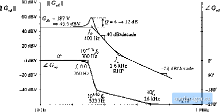

100 Вг

1 кНг

10 kHz

100 кНг

Fig. 8,33 Bode plot of tlic cotitro1-to-OLtput transfer function G ,;, buck-boost converter example, Phase rtivcrsal owing 10 ntitpuf voltage hversioti is not included.

20 (IB OdB -20 dB -40 dB -GOdB -SOdB

10 Hz

100 EIz

1 kHz

-180* -270-

10 kHz

too kHz

Fig. 8.34 Bode plot of the line-to-output transfer function C, buck-boost coiiverier example Phase reversal owing to output voltiije rwersal is not iiieluded.

ТяЫе iL2 Salieiil teatures of the small-siunal CCM ttansfer functions of some basic dc-dc converters

8.2.2 Transfer Functions of Some Basic CCM Converters

The salient features of the line-to-output and controi-to-output transfer functions of the basic buck, boost, and buck-boost converters are summarized in Table S.2. In each case, the control-to-output transfer function is [)f the form

and the line-to-output transfer function is of the form

(S.l 32)

(8,133)

The boost and buck-boost converters exhibit control-to-output transfer functions containing two poles and a right half-plane zero. The buck converter Gj,(*) exhibits two poles but no zero. The line-to-output transfer functions of all three ideal converters contain two poles and no zeroes.

These results cim be easily adapted to transformer-isolated versions of the buck, boost and buck-boost converters. The transfonner has negligible effect on the transfer functions С (л) and ОД,), other than introduction of a turns ratio. For example, when the transformer of the bridge topology is driven symmetrically, its magnetizing inductance does not contribute dynamics to the converter small signal transfer functions. Likewise, when the transf[)rmer magnetizing inductance of the forward con verter is reset by the input voltage v, as in Fig. 6,23 or 6.2S, then it also contributes negligible dynamics In all transformer-isolated converters based on the buck, boost, and buck-boost converters, the line-to output transfer function should be multiplied by the transformer turns ratio; the transfer functions

(8.132) and (8.133) and the parameters listed in Table 8.2 can otherwise be directly applied.

8.2.3 PhjsicaJ Origins of tht Right Half-Plant; Zero in Converters

Figure 8.35 contains a block diagram that illustrates the behavior of the right half-plane zero. At low frequencies, the gain (s/ft)) has negligible magnitude, and hence = At high frequencies, where the