30 dBQ 60 dBQ 40 dBQ 20 dBQ OdBQ

-20 dBQ

10 ь loon

ICQ 1Й 0.1 Q

100 Hi

1 kHi

10 kHz

100 kHz

1 MHz

Fig. 8,40 ConsiruKtion of the composite asymptotes of Z . The asymptotes of the series combination can be approximated by simply .selecting the larger of the individual resistor and capacitor asymptote.4.

In terms of freqtieticy / this occurs at

(8,138)

So the capacitor impedance magnitude is a line with slope -20 dB/dec, and which passes through OdBQ at 159 kHz, as shown in Fig, 8.39. It should be noted that, for simplicity, the asymptotes in Fig. 8.39 have been labeled R and 1/oC. But to draw the Bode plot, we must actually pk>t dB£i; for example, 20 logij, (R/\ Q.) and 20 logi ((l/coQ/l Й).

Let us now consU-uct the magnitude of Z{s), given by Eq, (8.135). The magnitude of Z can be approximated as follows:

R-

R for R :s> UiJ}C

forj/tuc

(8,139)

The asymptotes of the series combination are simply the larger of the individual resistor and capacitor asymptotes, as illustrated by the heavy lines in Fig. 8.40. For this example, these are in fact the exact asymptotes of In the limiting case of zero frequency (dc), then the capacitor tends to an open circuit. The series combination is then dominated by the capacitor, and the exact function tends asymptotically to the capacitor impedance magnitude. In the limiting case of infinite frequency, then the capacitor tends to a short circuit, and the total impedance becomes simply R. So the R and l/tdC lines are the exact asymptotes for this example.

The corner frequency/q, where the asymptotes intersect, can now be easily deduced. At angular frequency Щ = 2я/о, the two asymptotes are equal in value:

(8,140)

Solution for й)ц and leads to:

8.3 Graphical Conatrticlion of Impedances and Transfer function.s

(S.140

So if we tan write analytical expressions for the asymptotes, then we ean equate the expressions to find analytical expressions forthe corner frequencies where the asymptotes intersect.

The deviation ofthe exact curve frotn the asymptotes follows all ofthe usual rules. The .slope of the asymptotes changes by +20 dB/decade at the corner frequency/ц (i.e., frotn -20 dBSi/decade to 0 iBSi/decade), and hence there is a zero at / = fy So the exact curve deviates frotn the asymptotes hy +3 dBQ at/=4 and by +1 dBQ at/= 2f and at/= J(fl.

SerJES Resonant Circuit Example

As a second example, let us construct the magnitude asymptotes for the series R~L-C circuit of Fig. S.41. The series itnpednnce Z(s) is

(8.142)

The magnitudes of the individual resistor, inductor, and capacitor asymptotes are plotted in Fig. 8.42, forthe values

fi = 1 k£l L= ImH С = 0,1цР

(8.143)

-►

Fig, SAl Series R-iC network exatnple.

The series impedance Z(.t) is dominated by the capacitor at low frequency, by the resistor at mid frequencies, and by the inductor at high frequencies, as ilhtstrated by the bold line in Fig. 8.42. The itnpedance Zu) contains a zero at angular frequeticy (0], where the capacitor and resistor asymptotes intersect. By equating the expression.s for the resistor and capacitor asymptotes, we can find ш,:

Fig. 8.42 Graphical ton-sttuction of II Z Ii of the series R-J network of Щ. 8.41, for the element values spoci-ftedbyBq. (8.143).

100 dBQ

SO dsn

60 dBQ -

40 dBQ

20dBfi

OdBa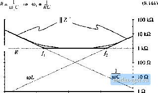

100 Hz

1 kHz

10 кНг

100 kHz

1 MHz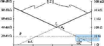

100 Hi

] kHz

10 kHz

100 kHz

1 MHz

Fig. 8.43 GriiphiL-iil toiLstriiclioii of inipedanL-e iisympiolcs tbr the series k-L-C network example, with R decreased ty JO W,

A second zero occurs at angular frequency Ц) where the inductor and resistor asymptotes intersect. Upon equating the expressions for the resistor and inductor asymptotes at OJj, we obtain the following:

(K,I4S)

So simple expressions for ail important features of the magnitude Bode plot of Z{.\) can be obtained directly. It should be noted that Eqs. {8,J44) and (8.145) are approximate, rather than exact, expressions for the comer frequencies ш, and a). Equations (8.144) and (8.145) coincide with the results obtained via the low-g approximation of Sechon 8.1.7.

Next, suppose that the value of R is decreased to 10 Q. As R is reduced in value, the approximate comer frequencies Wj and tOj move closer together until, at Л = 100 £i, they are both 1(X) krad/sec. Reducing R further in value causes the asymptotes to become independent of the value of Я, as illustrated in Fig. 8.43 for Л = 10 ft. The Z asymptotes now switch directly from wL to i/Q)C,

So now there are two zert>es at И = At corner frequency и)ц, the inductor and capacitor asympttjtes are equal in value. Hence,

U) f,=

- 1

(8.146)

Solution for the angular corner frequency Щ leads to

1

(8.147)

At (j) = Щ, the inductor and capacitor impedances both have magnitude R, called the characteristic impedance.

Since there are two zeroes at 0) = (Оц, there is a possibility that the two poles could be complex conjugates, and that peaking could occur in the vicinity of ш = So let us investigate what the actual curve does at 0) = Щ. The actual value of the series impedance Z(;(U,]) is

Z(juio)=fl + jo)o +

(8.148)