100 dB0

80 dBQ

Graphical CotislriicUon of Inipcdatices cnid Transfer Funaions 307

100 Ш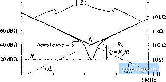

100 Hi

IkHi

10 kHz

100 kHz

Fig. 8.44 Actual impedance magnitude (solid line) Cor ilie series resonant R-L-C example. The inductor and capacitor impedances cancel out at/=and hence Z(/dJ) - Й.

Substitution ofEq. (8.14Й) into Eq. (8.147) leads to

(Й.149)

At (ii = (%, the itiductor and capacitor impedances ai-e equal in magnitude but opposite in phase. Hence, they exactly cancel out in the series impedance, and we are left with Z(jU)(,) = Л, as illustrated in Fig. 8.44. The actual curve in the vicinity of the resonance at ы = ш can deviate significantly from the asymptotes, because its value is determined by R ratherthan (OLor l/toC.

We know from Section 8.1.6 that the deviation ofthe actual curve from the asymptotes at (U = (Ofj is equal to Q. From Fig. 8.44, tme can see that

lano

(8. ISO)

(8.151)

Equations (8.146) to (8.151) are exact resuhs for the series resonant circuit.

The practice of adding asymptotes by simply selecting the larger asymptote can be applied to transfer functions as well as impedances. Forexample, suppose that we have already constructed the magnititde asymptotes of two transfer functions, G, and Cj, and we wish to find the asymptotes of G = Gi + Gj. At each frequency, the asymptote for С can be approximated by simply selecting the larger of the asymptotes for G, and G:

f;,*G,

(8.152)

Corner frequencies can be found by equating expressions for asymptotes as illustrated in the preceding examples. In the next chapter, we will see that this approach yields a simple and powerful method for determining the closed-loop transfer functions of feedback systems.

8.3.3 Parallel Impedances: Inverse Addition пГ jlsymptutes A parallel combmatron represents inverse addition of impedances:

7 = L

(8.153)

If the asymptotes of the individual impedances Z Z, .... are Icnown, then the asymptotes of the parallel combination Z. can be found by simply selecting the smiillest individual impedance asymptote. This is true because the smallest impedance will have the largest inverse, and will dominate the inverse sum. As in the case of the series impedances, this procedure will often yield the exact asymptotes of Z

Let us construct the magnitude asymptotes for the parallel /f~L-C network of Fig. 8.45, using the following element values:

K= lOii i= ImH С = 0.1 pF

(S.l54)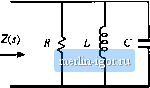

Impedance magnitudes of the individual elements are illustrated in Hg, 8.4S Farallel RLr-C tietwork Fig. 8.46. The asymptotes for the total parallel impedance Z are example, approximated by simply selecting the smallest individual element

impedance, as shown by the heavy line in Fig. 8.46. So the parallel impedance is dominated by the inductor at low frequency, by the resistor at mid frequencies, and by the capaciUtr at high frequency. Approximate expressions for the angular corner frequencies are again found by equating asymptotes:

atm = 03, R = {aL i = y at(0 = fflj, Д = -Ц

(8.135)

These expressions could have been obtained by conventional analysis, combined with the low-Q approximation of Section S.1.7.

FJg. 8.46 Construction of the composite a-symptotes of II ZII. for the parallel R-L-C example. The asymptotes of the parallel combination can be approximated by simply selecting the smallest of the individual resistor, inductor, and capacitor asymptotes.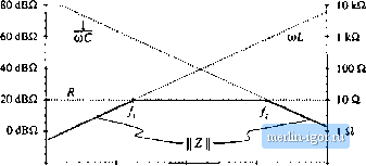

-20 dBQ

0,1 Q

100 Hz

1кНг

10 kHz

100 kHz

IMHz

S.. GiapiucBt Censmiaiim ofhnpedences and Тгапфг Fmciions

80 dBQ 60dBii

Fig. 8,47 Graphital construction of impedance asymptotes 40 dB£l for the parallel u-l-c example, with r increaseti to 1 V.q, 20 dBft

-20 dBQ

o.i a

100 Hz

1 kHz

10 kHz

100 kHi

1 MHz

8.3.4 Parallel Resonant Circuit Example

Figure 8.47 illustrates what happeti.4 when the value of Л m the parallel R~L-C network is increased to 1 кЙ, Tlie a.symptotes for ] Z tlieti bieconie independent of R, ;uid change directly from iiih to i/юС at angular frequency Olg. The comer frequency Щц is now the frequency where the inductor and capacitor asymptotes have equal value:

(8.156)

which implies that

(8.157)

At и = Шц, the slope of the asymptotes of IIZ changes from +20 dB/decade to -20 dB/decade. and hence there aie two poles. We should investigate whether peaking occurs, by determining the exact value

of IIZ Ij at (0 = Шц, as follows:

(3.158)

2(jt0o) = jt0ui

1

Substitution ofEq. (8.156) into (8.158) yields

Z(Mi) = T-7

R jR R R R Я

- = /f

(8.159)

So at Ы = Щ, the impedances of the inductor and capacitor again cancel out, and we are left with Z(j<i) = R. The values of L and С determine the values of the asymptotes, but R determines the value of the actual curve at fJ = dig.

The actual curve is illustrated in 8.48. The deviation of the actual curve from the asymptotes at (ii=0)o is