Fig. S.48 Aeiual impedance magnitude (snlid line) for the pai-allel R-LC example, The inductor and capacitor iiriped-ance.4 cancel out at / = and hetice Z(ycu,} = /;,

80 dsn

60dBn 40 dBQ 20 dBii OdBQ

-20 dBO

10 ш 1ш

100 i2 10 Й 1 Q 0.Ш

100 Ш

i kHz

10 kHz

100 kHz

I МНг

(8,160)

(8.161)

Equations (8.156) to (8.161) are exact resuh.s for the parallel resonaill circuit.

The graphical construction method for impedance magnitudes is well kntiwn, and reactance paper be purchased commercially. As illustrated in Fig. 8.49, the magnitudes of the impedances of various inductances, capacitances, and resistances are plotted on setnilogarithmic axes. .Asymptotes for the impedances of R-LC networks can be sketched directly on these axes, and numerical values of corner frequencies can then be graphically determined.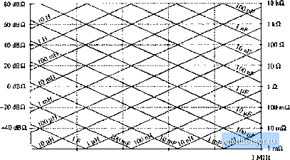

-iOdBfl

10 Hz

100 Нг

I tHz

10 kHz

100 kHz

Fig. 8.49 Reactance paper : an aid for graphical cunstfuctioii of impedances, with the magnitudes of various inductive, capucitive, and i-esistive impedances preplotted.

s.3 Giaphical Comtiucnim of bipeciances and Trmufer Funcliotis 311

His)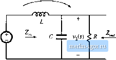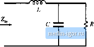

Fig. 8.50 Two-pole low-pass filter based on voliage divider circuii: (a) transfer function H{x), (b) determination of by setting independent sources id zero, (c) determination uf Zjfj).

8.3.5 Voltage Divider Transfer Fun<:tians: Division of Asymptutes

Usually, we can express transfer functions in terms of impedances-for example, as the ratio of two impedances. If we can construct these impedances as described in the previous sections, then we can divide to construct the transfer function. In this section, constniction of the transfer function H(s) of the two-pole R-L-C low-pass filter (Ftg. 8.50) is discussed in detail. A ftlter of this form appears in the cimonical model for two-pole coitverters, and the results of this sectioit aie applied in the converter examples of the next section.

The familiar voltage divider formula shows that the transfer function of this circuit can be expressed as the ratio of impedances Zj/Zj, where Z, =Zj -l-Zj is the network input impedance:

z, + z,

(R.162)

For this example, Zj(y) = sL, and Zj(j) is the parallel combination of Д and 1ЛС. Hence, we can find the transfer function asymptotes by constructing the asymptotes of Zj and of the .series combination represented by Zt and then dividing. Another approach, which is easier to apply in this example, is to multiply the numerator and denominator of Eq. (8.162) by Z,: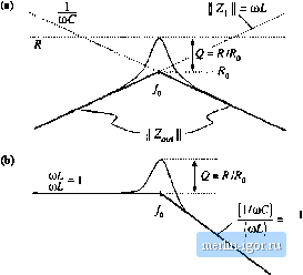

Fig. 8.51 Graphical cwistmclioii of HandZ ,of the vohage divider circuit: (a) output impedance Z (b) transfer function И.

4 )

(8,(63)

where Z - Z {{Z is the output impedance of the voltage divider. So another way to construct the voltage divider transfer function is to first construct the asymptotes for Z; and for the parallel combination represented by Z, and then divide. This method is useful when the parallel combination 7, \\ is easier to construct than the series combination Z, + Z. It often gives a different approximate result, which may be more (or sometimes less) accurate than the result obtained using Z, . The output impedance Z, in Fig. 8.5()(b) is

(3.164)

The impedance of the parallel K-L-C network is constructed in Section S.3.3, and is illustrated in Fig. 8.51 (a) for the high-Qca.se.

According to Eq. (S.163), the voltage divider transfer function magnitude is j = II Z, IK [ Z, . This quantity is constructed in Fig. 8.51(b). For ffl < [Oq, the asymptote of Z, [ coincides with II Zj : both iire equal to toL. Hence, the ratio is Z , / Z, = 1. For Ш > (i), the asymptote of Ц Z,, is ItoC,while II Zj is eqtial to (uL. The ratio then becomes Z , / Z, = I/mLC, and hence the htgh-

...... CUL FiK, 8.52 Effect of iiiciBasing L on the output

impedance asyinplotes, corner frequency, and