&5 Measurement of AC Transfer Functions and Impedances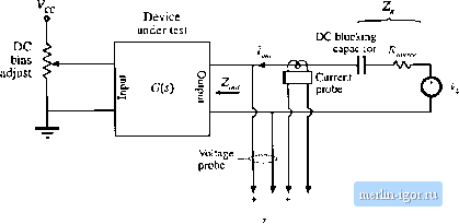

Fig. ЯМ Measui-etncm of tlie output irnfdaiiceor a ciivult.

voltage across the amplifier output impedance:

cs.nj)

A ciinent prohe is used to measure The current probe produces a voltage proportional tof ,; this voltage is connected to the networlt analyzer input \. A voltage probe is used to measure the amplifier output voltage P , The networli analyzer displays the tiansfer function i./ii. which is proportional loZ,ur Note that the value of and the amplitude of vj do not affect the measurement of Zonula power applications, it is sometimes necessary to measure impedances that are very small in magnitude. Grounding probleras[4] cause the test setup of Fig. 8.60 to fail in such cases. The reason is illustrated in Fig. 8.61 (a). Since the return connections ofthe injection source i; and the analyzer input are both cotmected to earth gr[)uiid, the injected current can return to the source through the return connections of either the injection source or the voltage probe. In practice, divides between the two paths according to their relative impedances. Hence, a significant current (1 - k) flows through the return connection ofthe voltage probe. If the voltage probe return connection has some total contact and wiring impedance Z , then the current induces a voltage drop (1 - t),2j t,t he vohage probe wiring, as illustrated in Fig. 8.61(a). Hence, the network analyzer does not correctly ineasure the voltage drop across the impedance Z. If the internal ground connections ofthe network analyzer have negligible impedance, then the network analyzer will display the following impedance:

Z + (1 - l)Z ,.= 2 + Z iJZ

(8.180)

Here, Zj is the impedance of the injection source return connection. So to obtain an accurate measurement, the followins; condition must be satisfied:

(8.181)

Impedance under test

ZCi)

Injection

source

connection

ow ml

Voltage probe -

Valtage protie ,.* (leiurn connectioti

1-Ih

Net wotic Analyzer

Injection source

Measured inputs

Impedance under lest

Zis)

Injection source return connection

Voltage probe

Voltage probe return connection

1 :n о

-ОШ-W

Network Attalyzer

Injection source

Measured inputs

-0 +

Fig. 8.61 Measiiremeat of Et small impedance /.(s): (a) current flowing in tlie return connection of the voltage р1Ч)Ье induces a vohage ditip that corrupts tho measureineiii; (b) an Inipioved experiment, irieorpuratitig isolation of the injection source.

A typical Itjwer litnit on Z ( is a few teas oi liundieds of milliohms.

An improved test setup for measurement of small impedances is illustrated in Fig. 8.61(b). An isolation transfortner is inserted between the injection source and the dc blocking capacitor. The return ctmnections of the voltage probe and injectitm source are no longer in parallel, and the injected current inust now return entirely thrtmgh the injection source return connection. An added benefit is that the transfonner turns ratio n can be increased, to better match the injection source impedimte to the impedance under test. Note that the impedances of the transformer, of the bl[)cking capacitor, and of the probe imd injection source teturn c[)nnections, do not affect the tneasuretnent. Much sinaller itnpedances can therefore be tneasuied using this itnproved approach.

8.6 SUMMARY 0¥ KEY POINTS

1. The miinituJe Bode diagrdms of funetlons whieh vary as (J/fflf have slopes equal to 20i dB per detade, and pass through 0 dB at =/n.

2. It is gcKxl practioe to express transfer functions in normalized pole-zero form; this form direetly exposes expressions for the sahenl features ofthe response, that is, the corner frequencies, reference gain, ett.

3. The right half-plane zero exhibits the magnitude response of the left half-plane zero, but the phase response of the pole.

4. Poles and zeroes tan be expressed in frequenty-inverted form, when it is desirable to refer the gain to a hlgh-frequeney asymptote.

5. A two-pole response t:an be written in the standard normalized form t>f Eq. (8.58). When Q > 0.5, the poles are complex conjugates. The magnitude response then exhibits peaking in the vieinity ofthe comer fre-queney, with an exact value of Q at/=/Q. High Q also eauses the phase to ehange sharply near the corner frequency.

6. When Q is less than 0.5, the two pole response tan be plotted as two real poles. The lov/-Q approximation preditls that the two poles ottur at frequencies /Q and Q/]y These frequencies are within 10% ofthe exact values for Q 0,3

7. The ]av/-Q approximation tan be extended to find approximate roots of an arbitrary degree polynomial. Approximate analytital expressions for the salient features cnn be derived. Numerical values are used to justify the approximations.

8. Salient features of the transfer functions uf ihe buck, boost, and butk-lmosl converters are tabulated in Section 8.2.2. The line-to-output transfer functions of these converters contain two poles. Their control-to-outpul transfer functions contain two poles, and may additionally tontain a right half-plane zero.

9. Approjtinnate magnitude asymptotes of impedances and transfer functions can be easily derived by graphical construction. This approach is a useful supplement to conventional analysis, because it yields physital insight into the circuit behavior, and because il exposes suitable approximations. Several examples, including the impedances of basic series and parallel resonmt circuits and the transfer function H{s) ofthe voltage divider circuit, are worked in Section 83. The input impedance, output impedance, and transfer functions of the buck convener are constructed in Section 8.4, and physical origins of ihe asymptotes, corner frequencies, and g-factor are found.

10. Measurement of transfer funttions and impedances using a network analyzer is discussed in Secuim 8.5. Careful attention to ground connections is important when measuring small impedances.