9.4 Stahihry

-90-

-180-

-270-

Fig. 9.10 Magnitude .ind phase asymptotes for the loop gain Tof Eq. (9.21),

become worse (higher 2. longer ringing) until, for (p, :Ё 0, the system becomes unstable.

Let us consider a loop gain T\.<} which is well-approximated, in the vicinity of the crossover frequency, by the following function:

1 > ..f-

<921)

Magnitude and phase asymptotes are plotted in Fig. 9.10. This function is a gotxl approximation near the crossover freqtiency for many common loop gains, in which T J approaches unity gain with a -20 dB/decade slope, with an additional pole at frequency/j = iHjUK. Any additional poles and zeroes are assumed to be sufficiently far above or below the crossover frequency, such that they have negligible effect on the system transfer functions near the crossover frequency.

Note that, as/j -* oo, the phase margin approaches 90°. As 0, ф + 0°. So as i.s reduced, the phase margin is also reduced. Lets investigate how this affects the closed-loop response via Г(1 -I- T). We can write

T(.()

* t(j) ts еръ

using Eq. (9.21). By putting this into the standard itormalized quadratic form, one obtains

m 1

where

(9.22)

(9.23)

40(1Bt

Fig. 9.11 Cojistfuction of 2 I -20dB/decafe magnitude asymptotes of tJie closed-loop transfer function OdB

77(1 -I- 7), for tiie bvi-Q case.

-20 dB

-40 dB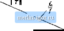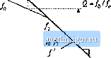

-40 dB/decade

So the closed-loop response contains quadratic poies at/., the geomettic mean of f, and . Tliese poies have a low Q-factor when/ц -й;/j. In this case, we can use the low-g approximation to estimate their frequencies:

Cw, = tau

(g.24)

Magnitude asymptotes are plotted in Fig. 9.11 for this case. It can be seen that these asymptotes conform to the rules of Section 9.3 for constructing T/(] +Т) by the algebra-on-the-graph method.

Next consider the high-Q case. When the pole frequency/2 is reduced, reducing the phase margin, then the 2-factor given by Eq. (9.23) is increased. For Q > 0.5, resonant poles occur at frequency /.. The magnitude Bode plot for the case</(, is given in Fig. 9.12. The frequencycontinues to be the geometric mean of/2 and, and/ now coincides with the crossover (unity-gain) frequency of the ГЦ asymptotes. The exact value of the closed-loop gain T/(l + T] at frequency /1 is equal to Q = fjfi.- As shown in Fig. 9.12, this is identical to the value of the low-frequency -20 dB/decade asymptote (JqIJ), evaluated at frequency/,. It can be seen that the Q-factor becomes very large as the pole frequency is reduced.

The asymptotes of Fig. 9.12 also follow the algebra-on-the-graph rules of Section 9.3, but the deviation of the exact curve from the asymptotes is not predicted by the algebra-on-the-graph method.

£OdB

Fig. 9.12 Construction of magnitude asymptotes of die closed-loop transfer function T/(i + T), for the high-C сак.

e=jy........

40 dB/decade

2QdB i5 dB 10 dB 5dB OdB -5dB -lOdB -15 dB -20 dB

0= iCr 20° 30° 40 50° 60 70 80° 90°

Fig. 9.13 Relationship between loop-gain phase margin (p, and closed-loop peaking factor Q.

These two poles with -factor appear in bioth 77(1 -i- T) and 1/(1 -i- 7. We need an easy way to predict the 2-factor. We cim obtain sueh a relationship by finding the frequency at which the magnitude of Tis exiittly equal to unity. We then evaluate the exact phase of Tat this frec[uency, ;md compute the phase margin. This phase margin is a function ofthe ratio /q ;, or Q. We can then solve to find Q as a function ofthe phase margin. The result is

sm Ф Ф, = tan

(9.25)

This function is plotted in Fig. 9.13, with Q expressed in dB. It cim be seen that obtaining real poles (Q < 0.5) requires a phase margin of at least 76°. To obtain Q - \, -d phase margin of 52° is needed. The system with a phase margin of 1° exhibits a closed-Uxip response with very high Q\ With a small phase margin, TXjbi) is very nearly equal to -1 in the vicinity ofthe crossover frequency. The denominator (l+T) then becomes very small, causing the closed-loop transferfunctions to exhibit a peaked response at frequencies neiir the crossoverfrequency

Figure 9.13 is the result for the simple loop gain defined by Bq. (9.21). However, this loop gain is a gtxxi approximation for many other loop gains that are encountered in practice, in which Ц T approaches unity gain with a-20 dB/decade slope, with an additional pole at frequency/j. If all other poles and zeroes [)f Т(.ч) are sufficiently fiir ab[)ve or below the crossover frequency, then they have negligible effect on the system transfer functions near the crossover frequency, and Fig. 9.13 gives a good approximation for the relationship between (p, and Q.

Another common case is the one in which T \\ approaches unity gain with a -40 dB/decade slope, with an additional zero atfrequency /j. As/j is increased, the phase margin is decreased and Q is increased. It can be shown that the relation between tp and Q is exactly the same, Ec[. (9.25).

A case where Fig. 9.13 fails is when the lotjp gain Дs) three or more poles at or near the cross-