2 ЛЛг-

ТППП

ТППГ

Section 2

ЛЛг-

ПППГ

ТЛПГ

Section 1

Fig, 10.25 TXvii-.sectiun input filt&r example, empluying itj-Lf, parallel damping iu each seeticm.

10.4.5 Example: Two Stuge Input Filter

As an example, let us eonsider the design of a two-stage filter using R-L parallel damping in each section as illustrated in Fig. 10.25 [17]. It is desired to achieve the same attenuation as the single-section filters designed in Sections 10.3.2 and 10.4.1, and to filterthe input current of the same buck converter example of Fig. 10.8. These filters exhibit an attenuation of SO dB at 250 kHz, and satisfy the design inequalities ofEq. (10.13) with the 2, and [ Zy\\ impedances of Fig. 10.10. Hence, lets design the filter of Fig. 10.25 to attain 80 dB of attenuation at 250 kHz.

As de.sctitied in the previous section aud below, it is advantageous to stagger-tune the filter sections so that interaction between filter sections is reduced. We will find that the cutoff frequency of filter section 1 should be chosen to be smaller than the cutoff frequency of section 2. In consequence, the attenuation of section 1 will be greater than that of section 2. Let us (somewhat arbitrarily) design to obtain 45 dB of attenuation from section 1, and 35 dB of attenuation from section 2 (so that the total is the specified SO dB). Let us also select = = n = i-/i-y = 0.5 for each section; as illustrated in Fig. 10.23, this choice ieads to a g(k)d compromise between damping of the filter resonance and degradation of high frequency filter attenuation. Equation (10.3S) and Fig. 10.23 predict that the /fy-£ damping network will degrade the high frequency attenuation by a factor of (1 + 1/л) = 3, or 9.5 dB. Hence, the section 1 undamped resonant frequency ffi should be chosen to yield 45 dB + 9,5 dB = 54.5 dB => 533 of attenuation at 250 kHz. Since section 1 exhibits a two-pole (- 40 dB/decade) roll-off at high frequencies, ffi should be chosen as follows:

(10.46)

Note that this frequency is well above the 1.6 kHz resonant frequency/) of the buck converter output filter. Consequently, the output impedance II Z, can be as large as 3 Q, and still be well below the 11 Zdm) II and II Zt,(/to) plots of Fig. 10.10

Solution ofEq. (10.37) for the required section 1 characteristic impedance that leads to a peak Output impedance of 3 il with н 0.5 ieads to

V = J1==-== = 2.l2n (10.47)

У2 (1+2и) /2(0.S)[l+3(0.5))

The filter inductanee and capacitance values are therefore

L, = 5 = 31.2 rH

Ь> (10.48)

The section 1 damping network inductance is

7t., = 15.6iH (10.49)

The section 1 damping resistance is found from Eq. (10.34):

The peak output itnpedance will occur at the frequency given by Eq. (10.36), 15.3 kHz. The quantities II Z (/a)) II and 11 2д,(/ш) [ for fiiter section 1 can now be constructed analytically or plotted by computer simulation. II Z;(j(t)) is the section 1 input impedance Z,.[ with the output of section 1 shorted, and is given by the parallel combination ofthe sL and the iR + an-L) branches. Zijisi) \\ is the section 1 input impedance with the output of section 1 open-circuited, and is given by the seties cotnbination of Zi(.!) with the capacitor itnpedance \lsC. Figure 10.26 contains plots of Zj(/(i)) and Zl)(jьi) \\ for fiiter section 1, generated using Spice.

One way to approach design of filter section 2 is as follows. To avoid significantly modifying the overall fiiter output impedance Z , the section 2 output impedance ZJjfii) \ \ must be sufficiently less than [ Zf/fQoi) II and Z(/(i>) . It can be seen from Fig. 10.26 that, with respect to Zp(Ji) , this is most difficult to accotnplish when the peak frequencies of sections 1 and 2 coincide. It is tnost difficult to satisfy the Z,{j<ii) \\ design criterion when the peak frequency of sections 2 is lower than the peak frequency of section 1. Therefore, the best choice is to stagger-tune the fiiter sections, with the resonant frequency of sechon 1 being lower than the peak frequency of section 2. This itnplies that section 1 will produce tnore high-frequency attenuation than section 2. For this reason, we have chosen to achieve 45 dB of attenuation with section 1, and 35 dB of attenuation from section 2.

The section 2 undamped resonant frequency j should be chosen in the same manner used in Ec]. (10.46) for .section 1. We have chosen to select n = rt = LJLj = 0,5 for sectitm 2; this again means that the fij-L, dntnping network will degrade the high frequency attenuation by a factor of (1 + = 3, or 9.5 dB. Hence, the section 2 undamped resonant frequency should be chosen to yield 35 dB + 5.5 dB = 44.5 dB = 169 of attenuation at 250 kHz. Since section 2 exhibits a two-pole (- 40 dB/decade) roll-off at high frequencies, should be chosen as follows:

fp .. 19.25 (10.51)

The output impedance of section 2 will peak at the frequency 27.2 kHz, as given by Eq. (10.36). Hence, the peak frequencies of sections 1 and 2 differ by aitnost a factor of 2.

20dBii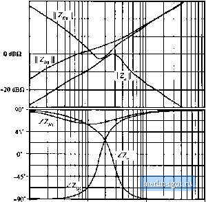

1 kHz

in kHz

1 МНг

Fig. 10.26 Bode plot of Zi atid Zj,j for filter section 1. Also sliowti is tlte Dode plot for the output impedatice of filter section 2,

Figure 10,26 shows that, at 27,2 kHz, HZyjC/O)) has a magnitude of roughly Э dBQ, and that Zyy;(/tfl) ll is approximately 7 dB£2, Hence, let us design section 2 to have a peak output impedance of OdBfi =Ф 1 q. Solution ofEq. (10.37) for the required section 2 characteristic impedance leads to

Rnsi =

II mm

1 £1

2ftjl+2ny yj2ifi.5)\L + 2(0.5) The section 2 element values are therefore

= 0.71fi

(10.52)

rt/,j=2.9

= 11.7 iiF

(10.53)

j - - Rt

3 + 4л l + Zu

=0,65S2

2 1 + 4h

A Bode plot of the resulting Z is overlaid on Fig. 10.26. It can he seen that ZJJlii) is less than, but very close to, Zpj(/co) between the peak frequencies of 15 kHz and 27 kHz. The impedance inequalities (10.45) are satisfied somewhat better helow 15 kHz, and are satisfied very well at high frequency.

The resulting filter output impedance l Z,(/to) is plotted in Fig. 10.27, for section 1 alone and for the complete cascaded two-section filter. It can be seen that the peak output impedance is approxi-