AC and DC Equivalent Circuit Modeling of the Discontinuous Conduction Mode

So far, we have derived equivalent eireuir m[)dei.4 for dc-dc pulse-width modulation (PWIVI) converters operating in the continuous conduction mode. As illustrated m Fig. 11.1, tlie basic dc conversion property is modeled by an effective dc transformer, having a ttirns ratio equal to the conversion ratio Мф). This model predicts that the converter has a voltage-source output characteristic, such that the output voltage is essentially independent of the load current or load resistance R. We have aLso seen how to refine this model, to predict losses and efficiency, converter dynamics, and small-signal ac transfer functions. We found that the transfer functions ofthe buck converter contain two low-frequency poles, owing to the convetter filter inductor and capacitor. The control-to-output transfer functions of the boost and buck-boost converters additionally contain a right half-plane zero. Finally, we have seen how to utilize these results in the design of converter control systems.

What are the basic dc and small-signal ac equivalent circuits of converters operating in the discontinuous conduction mode (DCM)? It was found in Chapter 5 that, in DCM, the output voltage becomes load-dependent: the conversion ratio MiD, K) к d function of the ditnensioniess parameter К - 2L/RT, which in turn is a function ofthe load resistance R. So the converter no longer has a voltage-source output characteristic, and hence the dc transformer model is less appropriate, hi this chapter, the averaged switch modeling [1-8] approach is employed, to derive equivalent circuits of the DCM switch networli.

In Section 11.1, it is .shown that the loss-free resistor model [9-11] is the averaged switch inodel of the DCM switch network, This equivalent circuit represents the steady-state and large-signal dynamic characteristics of the DCM switch network, in a clear and simple manner. In the discontinuous conduction mode, the average transistor voltage and current obey Ohms law, and hence the transistor is modeled by an effective resistor R,. The average diode voltage and current obey a power source characteristic, with power equal to the power effectively tlissipated in /(.Therefore, the diode is modeled with a dependent power source.

e(sAs) ,

-1 i- flbO >-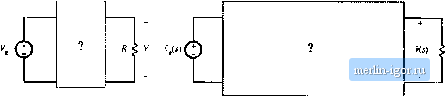

Fig. 11,1 The ol-yectivi; of this cliaptci- is ilie (Ictivutitm of large-Kignal md small-.4ignal iic equivaleni ciicuii models for conveners operating in the discontinuous conduction nrode.

Since most converters operate in discontinuoits conduction mode at some operating points, small-signal ac DCM models are needed, to prove tliat the control systems of such converters are correctly designed. In Section 11,2, a small-signal model of the DCM switch network is derived hy linearization of the loss-free resistor model. The transfer functions of DCM converters are quite different from their respective CCM transfer functions. The hasic DCM buck, boost, and buck-boost converters essentially exhibit simple single-pole transfer functions [12, 13], in which the second pole and the RHP zero (in the case of boost and bttck-boost converters) are at high frequencies. So the basic converters operating in DCM are easy to control; for this reason, converters are sometimes puфosely operated in DCM for all loads. The transfer functions of higher order converters such as the DCM Cuk or SEPIC are considerably more complicated; but again, one pole is shifted to high frequency, where it has negligible practical effect. This chapter concludes, in Section 11.3, with a discussion of a more detailed analysis used to predict high-frequency dynamics of DCM converters. The more detailed analysis predicts that the high-frequency pole of DCM converters occurs at frequencies near or exceeding the switching frequency [2-6]. The RHP zero, in the case of DCM buck-boost and boost converters, also occurs at high frequencies. This is why, in practice, the high-frequency dynamics can usually be neglected in DCM.

11.1 DCM AVERAGED SWITCH MODEL

Consider the buck-boost converter of Fig. 11.2. Let us follow the averaged switch modeling approach of Section 7.4, to derive an equivalent circuit that models the averaged terminal waveforms of the switch network. The general two-switch network and its tertninalquantities V(f). i](f), гЮ. and t;(r) are defined as illustrated in Fig. 11.2, consistent with Fig. 7.39(a). The inductor and switch network voltage and current waveforms are illustrated in Fig, 11.3, for DCM operation.

The inductor current is equal to zero at the beginning of each switching period. During the first subinterval, while the transistor conducts, the inductorcurrent increases with a slope of f (f)/L. At the

Swiich neiwork

Fig, 11,2 Buck-brtost convener example, with .switch nelwoik leminal qiimilitie.s ideiitilicd.

end of the first subinterval, the inductorcurrent i,f() attains the peak value given by

(11.1)

During the second subinterval, while the diode conducts, the induclor Current decreases wilh a slope equal to t-(r)/L. The second subinterval ends when the dittde becomes reverse-biased, at time f = (d f-rfj)/,. The inductor ctirrent then remains at zero for the baiance of the switching period. The inductor vtdtage is zero during the third subinterval.

A DCM averaged switch model can be derived with reference to the waveforms of Fig. 11.3. Following the approach of Section 7.4.2, let us find the average valties ofthe switch networli tenninal wavefonns l[(f), vil), iO). and in terms of the converter state variables (inductor currents and capacitor voltages), the input voltage f(/), and the subintervai lengths dj and rfj-

The average switch networlt inptit vttitage or the average tmnsisior voltage, is found by

averaging the v(t) waveform of Fig. 11.3:

{v,0)),-d,{tyud,i j(v(f)),-(v(0),J +rf,(() (v,(r)) Ше of the identity rf-{f) = 1 -(f,(r) -yj(() yields

Simiiar analysis leads to the following expression for the average dittde voltage:

(11.2)

(11.3)

{v,(r)) = rf,(r)[(v,(r)) - (v(/)).,. + dit) 0 + rf,(0[- {v(t)) = d, ){v,(t])-[ld,{t)){m)r

(11.4)

The average switch netwttrk inptit ctirrent {(t)) is found by integrating the i[(f) waveform of Fig. 11.3 over one switching period: