P(f)

big. 11.5 The dependem power source: (a) sehemabt symbol, (b) i-v eharaeteristic,

ber of common power-processing applications, including switch networlta operating in the discontinuous conductitm mode.

The pttwer source characteristic illustrated in Fig. 11.5(b) is symmetrical with respect to vtdtage and current; in consequence, the pttwer source exhibits several unique properties. Similar to the voltage source, the ideal power sotirce must not be short-circuited; otherwise, infinite current ttccurs. And similar to the cunent source, the ideiil power source must not be open-circuited, to avoid infinite terminal voltage. The power stmrce must be connected to a load capable of absorbing the power/?(r), and the operating point is defined by the intersection ofthe load and power source i-v characteristics.

As illustrated in Fig. ll.fi(a), series- and parallel-connected power sources can be combined

Fig, 11.Й Citv;uiE manipulations of power source elements: (a) cotnbination of series- and parallel- connected power sources into я single equivalent power source, (b) invariancii of the power source to reflcciiun through an ideal transformer of arbitrary turns isitio.

(a) ........ ......................Jii)

Fig, 11.7 (a) the Eeneral two-swilcti riolwork, and (b) the torrespoiiditig averaged switch imidel in the discciiitiiiu-ous conductioti mode: the average transistor wavefortns obey Ohms law, while the average diode waveforms hchave h5 a depeiident poww soutee.

into a single power stmrce, equal to the sum of the powers of the individual sources. Fig. ll.fi(b) illustrates how reflection of a power source through a transformer, having an arbitrary turns ratio, leaves the power source unchanged. Power sources are also invariant to duality transformations.

The averaged large-signal model of the general two-switch network in DCM is illustrated in Fig. 11.7(b). The input port behaves effectively as resistance R. The instantaneous power apparently consumed by is transferred to the output port, and the output port behaves as a dependent power source. This lossless two-port network is called the ioss-free resistor model (LFR) [9]. The loss-free resistor represents the basic power conversion properties of DCM switch networks [11]. It can be shown that the loss-free resistor models the averaged properties of DCM switch networks not only in the buck-boost converter, but also in other PWM converters.

When the switch network of the ЕЮМ btick-boost converter is replaced by the averaged model of Fig. 11.7(b), the converter equivalent circuit of Fig. 11.8 is obtained. Upon setting all averaged waveforms to their quiescent values, and letting the indtictttr and capacitor become a short-circuit and an open-circuit, respectively, we obtain the dc model of Fig. 11.9.

Systems containing power sources or lt)ss-free resistors can usually be easily solved, by equating average source and load powers. For example, in the dc network of Fig. 11.9, the powerflowing into the converter input terminals is

(11.23)

(,(0).

+ c:

Fig, I I.K Replacement of the switch network of the DCM buck-boost converter with the Itj.ss-frec resistor model.

Fig. 11,9 Dc netwoik exatnple ctiiirainmg a loss-free resistor tnotlei.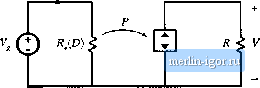

Tlie power flowing into tlie load resistor is

(11.24)

The loss-free resistor model states that these two powers mtist be equal:

Solution for the voltage conversion ratio M - V/V yields

---If.

(11.25)

(11.26)

Equation (11.26) is a general result, valid for any converter that can be modeled by a loss-free resistor and that drives a resistive load. Other arguments must be used to determine the polarity of V/V. In the bnclt-boost converter shown in Fig. 11.2, the diode polarity indicates that У/К, must be negative. The steady-state value of R is

where D is the quiescent transistor duty cycle. Substitution ofEq. (11.27) into (11.26) leads to

К V

DJ.R

< 11.27)

(11.28)

with 2/V7(T..This equation coincides with the previous steady-state result given in Table 5.2.

Similar arguments apply when the waveforms contain ac components. Forexample, consider the networlt of Fig. 11.10, in which the voltages and currents are periodic functions of time. The rms val-

Fig. 11.10 Ac network example ciiniaininE a loss-free re-sistor model.