120 V

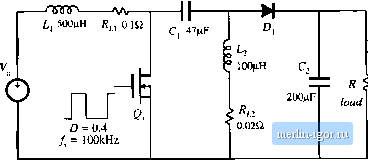Fig. 11,20 SEPlC example.

aodBV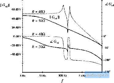

50 kHz

Fig. 11.21 Magnitude and pha.4c of the eoiitrol-to-mitput transfer fiiiiction oblaiuetl by siintikuloii of the SEPEC exatnple .shown in Fig. 11.20, for two viihics of the load resi.itiiiiee: fi = ЧОП when the eotiverter operates in DCM (solid liiie.s), and fi - 40fl for which die converter operates in CCM (diished lines).

the simulation setup are described in .Appendix B, Section B.2.1. Figure I 1.21 shows raagnititde and phase responses of the conhol-to-output transfer function obtained for two different values of the load resistance; A! =40 £2, for which the converter operates in CCM, and R - 50 i2, for which the converter operates in DCM. For these two operating points, the quiescent (dc) voltages and currents in the circuit are nearly the same. Nevertheless, the frequency responses are qualitatively very different in the two operating modes. In CCM, the converter exhibits a fourth-order lespon.se with two pairs of high-Q complex-conjugate poles and a pair of complex-conjugate zeros. Another RHP (tight-half plane) zero can be observed at frequencies approaching 50 kHz. In DCM, there is a dominant low-frequency pole followed

by a pair of complex-conjugate poles and a pair of complex-conjugate zeros. The frequencies ofthe complex poles aitd zeros are very close in value. A high-frequency pole and a RHP zert) cttntribiite additit)nal phase lag at higher frequencies.

11.3 HIGH-FREQUENCY DYNAIVHCS OF CONVERTERS IN DCM

As discussed in Section 11.2, transfer functions of converters operating in discontinuous conduction mode exhibit a dominant iow-freqtiency pole. A pole and possibly a zero caused by inductor dynamics, are pushed to high frequencies. To correctly model the high-frequency dynamics of DCM converters, one must account for the fact that the ac voltage across the inductor is not zero. Equation (11.12) is employed in Section 11.1 to greatly simplify the equations of the DCM averaged switch model. Although this model gives good restdts at low frequencies, it cannot accurately predict high frequency indtictor dynamics because it implies that the ac inductttr voltage is zero.

A more accurate approach is employed in this section. The subinterval length f/ is fotmd by averaging the inductorcurrent waveform ifj) of Fig. 11.3 [4-6]:

(11.64)

Solution for(V2(/) yields:

d2(t) =

-diO =

RXd){idit)).

(11.65)

Equation (11.65), together with Eqs. (11,3), (11,4), (11.7), and (11.10), constitutes a large-signal averaged inttdel in DCIVI that can be tised to investigate steady-state behavior, as well as low-frequency and high-frequency dynamics. Unfortunately, the model equations are more involved, and do not allow elimination of all converter voltages and currents in terms ofthe switch network average terminal waveforms.

Let us use this model to find predictions for the high-frequency pt>le caused by the inductor dynamics of DCM converters. Consider the btick-boost cttnverter of Fig. 11,2 having the DCM waveforms shown in Fig. 11.3, The average transistor voltage and the average diode current are selected as the switch network dependent variables. Substitution ofEq. (11.65) into Eq, (11.3) yields

, , и , , R,(r/){i (/))v(0). ,/(f)

ь(0),ч-(0)м,.-40(ИО) - - -J

(11.66)

The averaged switch voltage {Vf(f}}j. in Eq. (11,66) is a nonlinear function of the switch duty cycle, the average indtictor current, and the average input and otitput voltages:

(11.Й7)

A small-signal ac mttdel can be obtained by Taylor expansion ttfEq. (11.67), The small-signal ac component ofthe average switch voltage can be fotmd as:

А С and DC Equivalent Circuit Modeling of the Discontinuous Conduction Mode

+ It

Fig. 11.22 A small-signal ac motiel of the DCM buck-buust converter.

С R

(И.6В)

where the small-signal model parameters k, k, r, and/, are computed as partial derivatives of Vi evaluated at the quiescent operating point. In particular,

Substitution of Eq. (11.65) into Eq. (11.10) yields

(11.64)

ШтгШт,-{,.(0). dit)

The small-signal ac component i of the average diode current can be found as:

(11.70)

(ll.7t)

where the small-signal model parameters j, h., and are computed as partial derivatives of evaluated at the qtiiescent ttperating point. Figure 11.22 shows the small-signal ac model of the buck-boost converter, where the transistor and the diode switch are replaced by the sources specified by Eqs, (11.68) and (11.71), respectively. It can be sht)wn that this model predicts essentially the same low-frequency dynamics as the model derived in Section 11.2.

To find the control-to-output transfer function, we set = 0. At high frequencies, the small-signal ac component of the capacitttr voltage is very small, v = Ik Therefore, the contribution of the dependent source kj/ can be neglected at high frequencies. Then, from the equivalent circuit model of Fig. 11.22, we have

iLif,+г1Г;,-1-у,(/ = 0 iU.ll)

Equation (1 1.72) can be solved for the control-to-inductor current transfer function at high frequencies: