It tan be seen that this transfer function contains only one pole; the pole due to the Inductorhas been lost. The dc gain is now direcdy dependent on the load resistance r. In addition, the transfer function contains a right half-plane zero whose corner frequency is unchanged from the duty-cycle-controlled case. In genera], introduction of current programming alters the transfer ftinction poles and dc gain, but not the zeroes.

The line-to-output transfer functinn frjW is found by setting the control input i,. to zero, and then solving for the output voitage. The result is

i,.-Ci

r,\\R\

Substitution of the parameters for the buck-boost converter leads to

1 + .- M +D

Again, the inductor pole is lost. The output impedance is

ZJ,s]r\{R\\± For the buck-boost converter, one obtains

(12.4])

(12.42)

(12.43)

(12,44)

12,2,2 Averaged Switch Modeiing

Additional physical insight into the properties of current programmed converters can be obtained by use of the averaged switch modeling approach developed in Section 7.4. Consider the buck converter of Fig. 12.16. We can define the terminal voltages and currents of the switch network as shown. When the buck converter operates in the continuous conduction mode, the switch network average terminal waveforms are related as follows;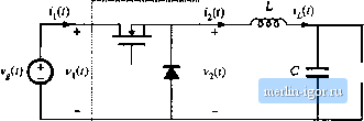

R < vii)

\ SwUeh network

Fig. 12.16 Averaged switch modeling of a current-programmed convetter: CCM buck exanipie.

(12.45)

We again invoke the approximation in which the inductor current exactiy follows the control current. In terms ofthe switch network terminal current ij, we can therefore write

The duty cycle dit) can now \x eliminated from Eq. (12.45), as follows:

(,-,С0), = 40(<ДО) = щ(Цг)), This equation can he written in the alternative form

(12.46)

(12.47)

(12.48)

Equations (12.46) and (12.48) are the desired result, which describes the average terminal relations of the CCM current-programmed buck switch network. Equation (12.46) states that the average terminal current {iiff}. is equal to the control current i\{t)).j.. Equation (12.4S) states that the input port of the switch network ctmsumes average power (p(()) equal to the average power flowing out ofthe switch output port. The averaged equivalent circuit of Fig. 12.17 is obtained.

Figure 12.17 descrihies the behavior of the current programmed buck converter switch network, in a simple and straightforward manner. The switch network output port behaves as a current source of value The input port follows a power sink characteristic, drawing power from the source equal

to the power supplied by the current source. Properties of the power source and power sink elements are descriled in Chapters 11 and 18.

Similar arguments lead to the averaged switch models ofthe current programmed boost and buck-boost converters, illustrated in Fig. 12.18. In both cases, the switch network averaged terminal waveforms can be represented by a current source of value {1,.(.С))т> in conjunction with a dependent power source or power sink.

A small-signal ac model of the current-programmed buck converter ciui now be constructed by perturbation and linearization of the switch network averaged temiiiiai waveforms. Let

Fig, 12.17 Averaged model of CPM buck convener.

Average/ wjteft network \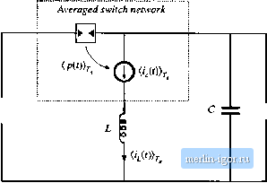

Iig. 12,ie Avei-aged models of CPM boost (a) and CPM buck-boost (b) converters, derived via averaged switch inodeling.

(.(0),]=V, + v,(i) (12,49)

(;2(0}, = /2 + .Vo (i,(0}, = /. + ?,(()

Perturbation and iitiearization of the (irCO)i-j current source of Fig. 12.17 simply leads to a cutrent source of value Perturbation of the power source characteristic, Eq. (12.48), leads to

(v, + o,(f))[/, +; i(/)) = + r,(r))( + f,(f)}

Upon equating the dc terms on both sides of this equation, we obtain

(12.50)

(12.SI)

The linear small-signal ac terms ofEq. (12.50) are