Fig, 12,23 Accuraw aeterminwitin of the Telalionship between the average inductor current and

rrtT,

JO

Tills is the more accurate relationship which is employed in this section.

A small-signal current programmed controller model is found by perturbation and linearization of Eq.( 12.59). Let

(i..ft )),] = /, 4, d(t) = D + d{!) miO) = Mi+mi(0

Mij(:t)=Mj-i-ni,(r)

(12.60)

Note that it is necessary to perturb the slopes rn and trt since the inductor current slope depends ou the converter voltages according to Eq. (i2.!). For the basic buck, boost, and buck-boost converters, the slope variations are given by

Buck converter

Boost converter

ra, =

(12.61)

Buck-boost converter

ii=X

h is assumed that m does not vary: /м, = M. Substitution of Eq, (12.60) into Eq. (12.59) leads to

[/L+*JO) = (/. + r,(t))-M,J.JD-Kf(o}-+/?i,(0}(f> + f(f))-y(jW2 + u,(I))(d-(()) -S The fnst-otder ac terms ate

TiCr) = t%(!) - [iWX + D*f 1- 0М{Г,у{г) - Й,(0- mW f-3)

With use of the equilibrium relationship PM = DMj, Eq. (12.63) can be further simplified:

lble 13,2 Current progmtnnied coiitroilergains for basic conveners

f ,(r> = Ut) - MJAO -2 iW -2 (0

Finally, solution for d(t) yields

oX .

(12.64)

(12.65)

This is the actual relationship that the current programmed controller follows, to determine d(t) as a function of i*.((). v i W iirl mC)- Since the quantities №ii(/), and tnjd) depend tm vii) and v(r), according to Eq. (12.61). we can express Eq. (12.65) in the following form:

d{t)=F

f,(O- -/,P,W-/.0(O

(12.66)

where = XIMJ, Expressions for the gains f, and f, for the basic buck, boost, and btick-boost converters, are listed in Table 12.2. A functional block diagram of the current programmed controller, corresponding to Eq. (12.66), is constructed in Fig. 12.24.

Cunent programmed converter models can now be obtained, by combining the controller block

Hg, 12,24 Functional block diagram of the current programmed controller.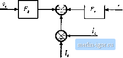

Ciirrtiil Pidgrammed Control

diagram of Fig. 12.24 with the averaged eonvetter models deiived itt Chapter 7. Figttre 12.25 illttstrates the CPM eottverter mttdeis t>btained hy tomhination of Fig. 12.24 with the buck, boost, and buck-boost models of Fig. 7.17. For each conveiter, the cuirent programmed controller contains effective feedback of the inductor cunent (t) and the output voltage v(0, as well as effective feedforward of the input voltage v{t),

12.3.2 Solution of the CPM Transfer Functions

Next, let us solve the models of Fig. 12.25, to determine more accurate expressions for the control-to-output and iine-to-otitput transfer functions of curtent-programmed buck, bot>st, and buck-boost converters. As discussed in Chapter 8, the converter output voltage v can be expressed as a function of the duty-cycle ( /and input voitage v. variations, using the transfer functions G,Js) and G,J,s)

(12.b7)

In a .similar nnanner, the inductor cunent variation / can be expressed as a function of the duty-cycle d and input voltage variations, by defining the transfer functions G,.j{s) and G.Jx).

where the traitsfer functions GJs) and Gj{.s) are given by:

(12.68)

(a) Buck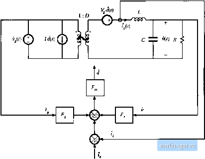

Fig. 12.25 More accurate models of currcnt-progninimed converteis; (a) Ixick, th) hoost, (c) buck-boost.