Area A

Fig. 13.2 The voltage v(t) induced in a loop of wire is relnted by Faradays law to the derivative ofthe total flux Ф(г) passing through the interior ofthe loop.

Flux Ф{0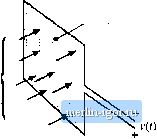

utiifortn flux distribution, we can express t(/) in terras of the tlux density B(f) by substitution of Eq. (13.4):

(13.6)

Thus, the voltage induced in a winding is related to the flux Ф and flux density В passing through the interior ofthe winding.

Len-s law states that the voltage v{t) induced by the changing flux Ф(() in Fig. 13.2 is of the polarity that tends to drive a current through the loop to counteract the tlux change. For exatnple, consider the shorted loop of Fig. 13.3. The changing tlux Ф(0 passing through the interior of the loop induces a voltage i(() around the loop. This voltage, divided by the impedance of the loop conductor, leads to a current ((f) as illustrated. The current/(f) induces a flux Ф{1), which tends to oppose the changes in Ф(/)- Lenzs law is involved later in this chapter, to provide a qualitative understanding of eddy current phenomena.

Amperes law relates the current in a winding to the magnetomotive force .IF and magnetic field H. The net MIVIF around a closed path of length is equal to the total current passing through the interior of the path. For example. Fig. 13.4 illustrates a magnetic core, in which a wire carrying current/(/) passes through the window in the center of the core. Let us consider the closed path illtistrated, which follows the magnetic field lines around the interior ofthe core. Amperes law states that

H-dl = total curretit passing through inteiior of path

(13.7)

The total current passing through the interior ofthe path is equal to the total current passing through the

Induced current

Fig, 13.3 lUusUatiun of Lenzs law in sl shorted loop of wire. The flux <D(r) induces cunent <(/), which in turn geuerates flux Ф(г) ibat tends to oppose changes in Ф(().

Них Ф(1)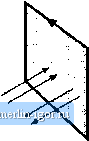

. Shorted loop

Induced flux Ф(0

Fig, 13.4 The net MMF around a closed piil.il is related by Amperes law to the total current pussins through the interior of the path.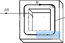

Magnetic path length L

window in the center of the core, or /(/). if the magnetic field is uniform and of magnitude H{t), then die integral is W(OCj for the example of Fig. 13.4, Eq. (13.7) reduces to

.#(t)=f/(t)i = <(f)

(13.8)

Thus, the magnetic field strength H(l) is related to the winding current ((f). We can view winding currents as sources of MMF. Equation (13.S) states that the MMF around the core, ./(0 /f(0£, . is equal to the winding current MMF /(/]. The total MMF around the closed loop, accounting for both MMFs, is zero.

The relationship between В and H, or equivalently between Ф and if, is determined by the core material characteristics. Figure 13.5(a) illustrates the characteristics of free space, or air:

(13,9)

The quantity fij is the permeability of free space, and is equal to 4я 10 Henries per meter in MKS units. Figure 13.5(b) illustrates the B-H characteri.stic of a typical iron alloy under high-level sinusoidal steady-state excitation. The characteristic is highly nonlinear, and exhibits both hysteresis md saturation. The exact shape of the characteristic is dependent on the excitation, and is difficult to predict for arbitrary waveforms,

For purposes of analysis, the core material characteristic of Fig. 13.5(b) is usually modeled by the linear or piecewise-iinear characteristics of Fig. 13.6. In Fig. 13.6(a), hysteresis and saturation are ignored. The B-H characteristic is then given hy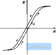

Fig. 13.S B-H chiliacteristics: (ii) of fi ее space or air, (b) of a typical inagnctic core itiateriiil.

Kig, 13,6 AppiDsiniatioi) of Ihe li-H charaeierisrics of a inagnelit core material: (a) by fiegleelitif; both hysteresis and saturation, (b) by neglecting hysteresis,

(13.10)

The core material permeability y. can be expressed as the product of tbc rciativc permeability and of Typical values of lie in the range 10 to 10\

The piecewise-linear model of Fig. 13.6(b) accounts for .saturation but not hysteresis. The core material saturates when the magnitude ofthe flux density В exceeds the saturation flux density B,. For \B \ < S. the characteristic follows Eq. (13.10). When B > B, f, the model predicts that the core reverts to free space, with a characteristic having a much sinaller slope approximately equal to Д. Square-loop materials exhibit this type of abrupt-saturation characteristic, and additionally have a very large relative permeability (i. Soft matetiais exhibit a less abrupt saturation characteristic, in which \i gradually decreases as И is increased. Typical values of are 1 to 2 Tesla for iron laminations and siii-cou steel, 0.5 to 1 Tesla for powdered iron and moiypermaiioy materials, and 0.25 to 0.5 Tesla for ferrite materials.

Unit systems for magnetic quantities are summarized in Table 13.1, The IVIKS system is used throughout this book. The imratioualized cgs system al.so continues to find .some use. Conversions between these systems are hsted.

Figure 13.7 summarizes the relationships between the basic electrical and magnetic quantities of a magnetic device. The winding voltage if) is related to the core flux and flux density via Faradays

Table 13,1 Units for magnetic quantities

Quantity

Unrationalized cgs

Conversions