We tan now determine the necessary core size. Evaluation ofEq. (14.52) yields

(l.724. 10-Q-cm)[l.07- 10-h)[i.77A)[i.5 a) (o.25T)*(1.5W)(0.3

= 0.049 cm

(14.76)

The smallest EE core listed in Appendix D that satisfies this inequality is the EE30, which has K = 0.0857 cm. The dimensions ot this cote are

A, 1.09 cin =

IV, 0.476 cm

MLT 6.6 cm

L, b.n cm

(14.77)

The air gap length is chosen according to Eq. (14.53):

[ап- 10-H/m](l,07- 10-h](i,5A) fo.25T)fl.09 cm}

0.44 mm

(14.78)

The number of winding 1 turns is chosen according to Eq. (14.54), as follows:

(l.07.10-h](i,5A] (0,2ST)[l.O9cm2) = .58.7 turns

(14.79)

Since an integral number of turns is requited, we round off this value to

(14.80)

To obtain the desired turns ratio, fij should be chosen as follows:

= (0 15)59 = 8,81

We asain round this value off, to

(14,82)

The fractions of the window area allocated to windings 1 and 2 are selected in accordance with Eq. (14.56):

/ 0.796 A = = 7 = 0.45

(1.77 j h ., (59J{l,77A

(14.83)

= 0.55

The wire gauges should therefore be

= 1.09 10 cm= - u.se #28 AWG

A <2 = 8.88- I0 cm2 -use#19AWG

(14.84)

The above American Wire Gauges are selected using the wire gauge table given at the end of Appendix D.

The above design does not accotmt for core ioss or copper ioss caused by the proximity effect. Let us compute the core loss for this design. Figiue Fig. 14.14 contains a sketch of the B-H кюр for this design. The tlux density B(f) can be expressed as a dc component (determined by the dc value of the magnetizing eitrrent Ij), plus an aC variation of peak amplitude AS that is determined by the current ripple Дг\(. The maximum value of 5(() is labeled В,; this value is determined by the sum of the dc component and the ac ripple component. The core material saturates when the apphed Bit) exceeds hence, to avoid saturation, B should be less than The core loss is determined by the amplitude of the ac variations in S(/) i.e., by Afi,

The ac component AB is determined using Faradays law, as follows. Solution of Faradays law for the derivative of B{t) ieads to

dt ПЛ

(14.85)

As illustrated in Fig. 14.15, the voltage applied during the first subinterval is VjJ,t) = V . This causes the

Fig. 14.14 B-H loop for the flyback transformer design example.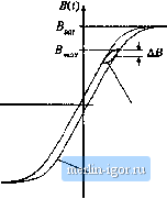

HJit)

Minor B-H loop, CCMfiyback eximple

B-H loop, lairge excittttion

Fig. 14.15 Variation of flux density Bit), flybatlt transformer example.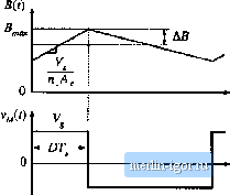

flux density to increase with siope

(14.86)

Over the first subintervai 0 < / < DTj., the flux density B(t) elianges by the net amount 2ДВ. This tiet change is equal to the slope given by Eq. (14.86), tnultipiied by the interval length fiT,:

л И,-у

Upon solving for ДД and expressing in cm, we obtain

ДД = - 10

(14,87)

(14.86)

For the flyback transformer exaraple, the peak ac flux density is found to be

10-*

(20QV}(0.4](6.67>t. Лд= ----

2[59)[l,09cm) = 0.041 T

(14.89)

To determine the core loss, we next exatnine the data provided by the manufacturer for the given core material. A typical plot of core loss is illustrated in Fig. 14.16. For the values of ДВ and switching frequency ofthe flyback transformer design, this plot indicates that 0.04 W will be lost in every cm of the core material. Of course, this value neglects the effects of harmonics on core loss. The total core loss Pj-j, will therefore tie equal to this loss density, miiitipiied by the volume ofthe core:

/>j., = [0.04W/cra3)(A,f )

= (0,04 W/cm)( 1.09 cm=)(5.77 cm) = 0.25 W

(14,90)

This core loss is less than the copper loss of 1.5 W, and neglecting the core k)ss is often warranted in designs that operate in the continuous conduction mode and that employ ferrite core tnateriais.