(15.6)

is the sum of the rms winding eurrents, referred to winding 1. Use of Eq, (15.4) to eliminate n, from Eq. (15.5) leads to

4Jf,.

jMLT)

(15.7)

The right-hand side of Eq. (15.7) is grouped into three tenns. The first group eontains speeifieations, while the second group is a function of the core geometry. The last tertn is a ftinction of AS, to be chosen to optitnize the design. It can be seen that copper loss varies as the inverse sqtiare of ЛЯ; increasing UB redtices Р,.

The increased copper loss due to the proximity effect is not explicitly accounted for in this design procedure. In practice, the proximity loss must be estimated after the core and winding geotne-tries are known. However, the increased ac resistance due to proximity loss can be accounted for in the design procedure. The effective valtie of the wire resistivity p is increased by a factor eqtial to the estimated ratio aJiii When the core geoinetry is known, the engineer can attempt to inipletnent the windings such that the estimated RaJdc is obtained. Several design iterations tnay be needed.

IS.1.4 Tutal power loss vs. ДВ

The total power loss f is found by adding Eqs. (15.1) and (15.7): The dependence of fj, and цОп iS is sketched in Fig. 15.3.

(15.B)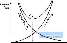

Optimum AB ДА

Hg. 15,3 Dependence of copper kiss, cure loss, and total loss on peak ac flux density.

IS.1.5 Optimum Flux Density

Let us now choose the value of ДВ that minimizes Ec[. (15.8). At the optimum ДВ, weeaii write

Mm d(M} dm)

Note that the optimum does not necessarily occur where P = P. Rather, it occurs where

dP..

rf(Afl) (/(ifl)

The derivatives of the core and copper losses with respect to ДЙ are given by

dihB)

4. = (l/:jAB)i-U,f,

(15.У)

(15,10)

(15.11)

(iS)

(15.12)

Substitution of Eqs. (15.11) and (15.12) into Eq. (15.10). and solution for AB, leads to the optimum flux density

plili, щт) ±

(15.13)

The resulting tutal power loss is found by substitution ofEq. (15.13) into (15.1), (15.S), and (15.9). Simplification ofthe resulting expression leads to

4/: W,Al This expression cait be regrouped, as follows:

(15.14)

ад- m]

(iWLr)£5f4

(15.15)

The terms on the left side ofEq. (15.15) depend on the core geometry, while the terms on the right side depend on specifications regarding the application (p, /, Я K, Р ,) and the desired core materiid [Kj, K-The left side ofEq. (15.15) can be defined as the core geometrical constant Kf:

S70 Transfonner Design

2 *\2

(15.16)

Hence, to design a transformer, the right side of Eq. (15.15) is evaluated. A core is selected whose K exceeds this value:

/f J> (15.17)

The quantity K is similar to the geometrical ctmstant u.sed in the previous chapter to de.4ign magnetics when core loss is negligible. is a measure of the magnetic size of a core, for applications in which core loss is significant. Unfortunately, K depends on % and hence the choice of core material affects the value of K-,. However, the P of гао.ч1 high-frequency ferrite material.s lies in the narrow range 2.6 to 2.8, and Кф varies by no more than ± 5% over this range. Appendix D lists the vaiues of Kj for various standard ferrite cores, fur the value P = 2.7.

Once a core has been selected, then the valties of A W f and MITare known. The peak ac ilux density ДВ can then be evaluated using Eq. (15.13), and the primary turns can be found using Eq. (15.4). The number of turns for the remaining windings can be computed using the desired turns ratios. The various window area allocations iue found using Eq, (14.35), The wire sizes for the various windings can then be computed as discu.ssed in the previous chapter,

fi.Wfpj (1518)

where Лу- is the wire area for winding j.

15.2 A STEP-BY-STEP TRANSFORMER DESIGN PROCEDURE

The procedure developed in the previous sections is summarized below. As in the filter inductor design procedure of the previou.4 chapter, this simple transformer design procedure should be regarded as a ffrst-pas.4 approach. Numerous issues have been neglected, including detailed insulation requirements, conductor eddy current losse.s, temperature rise, roundoff of number of turns, etc.

The following quantities are specified, using the units noted:

Wireeffecdve resisdvity p (il-cm)

Total rms winding currents, referred ш primary I - -y I

Desired turns ratios u/h, ij/Up etc.

v,(t)dt

Applied primary volt-seconds (V-sec)