Fig. 15.6 Wavefonns, CmV. converter tranafottner deaigti example.

Vl{0

Area X,

DT.

-ftV

nl.

n = H i2 = 5. The switching frequency is = 200 icHz, corresponding to = 5 s. A ferrite pot core consisting of Magnetics, Inc. P-material is to be used; at 200 kHz, this material is described by the following parameters: ЛГ, = 24.7 \УЯст\ P = 2.6. A fill factor of K = 0.5 is assumed. Total power loss of = 0.25 W is alloweil. Copper wire, having a resistivity of p = 1.724 10 il-cm, is to be used. Transfonner waveforms are illustrated in Fig. 15.6. The applied priinary volt-seconds are

1 = = (0.5) (5 psec) (25 V)

= Й2.5 V-ttscc

(15,25)

The primary rms current is

(15.26

It is assumed that the rms magnetizing current is much smaiier than the rms winding currents. Since the transformer contains only two windings, the secondary rms current is equal to

fj = )i/i = 20 A

The total rms winding current, referred to the primary, i.s

(15.27)

(15,2S)

The core size is evaluated using Eq. (15.19):

(1.72410- )(62.5- ]0 )(8)(24.7)il 4(0.5)(0,25)H )

(15.29)

= 0.00295

The pot core data of Appendix D lists the 2213 pot core with K, = 0.0049 for p = 2.7. Evaluation ofEq. (15.16) shows that K = 0.004? for this core, when p = 2.6. In any event, 2213 is the smallest standard pot core size having K < 0.00295.. The increased value of Л should lead to lower total power loss. The peak ac flux density is found by evaluation ofEq. (15.20), using the geometrical data for the 2213 pot core:

a(1.724-lQ-)(62.5-lQ-)\8) (4.42)

2C0..5) (0.297)(0.635)(3.15) (2.6)(24.7)

= 0.0858 Tesjii

1л.6)

(15.30)

This flux density is considerably less than the saturation flux density of approximately 0.35 Tesla. The primary tums are determined by evaluation of Et]. (15.21):

, 4 (62,5-10-)

2(ао858)((Ш5) (15.31)

= 5.74 tums

The secondary ttirns ate found by evaluation of Eq. (15.22). It is desired that the transformer have a 5:1 turns ratio, and hence

,.=1.15turns

In practice, we might select o, = 5 and ij = 1, This would lead to a slightly higher AB and slightly higher loss.

The fraction of the window area allocated to windings 1 and 2 are determined using Eq. (15.23):

(4 A\

= )-f = 0.5

( 1 ,15.33)

(i)(20A)

(8 A)

= 0.5

Forthis example, the window area is divided equally between the primary and secondary windings, since the ratio of their rms currents is equal to the turns ratio. We can now evaluate the primary and secondary wire area.s, via Eq. (15.24):

(0.5)(0.5)(0.297)

(5) (15.34)

A i J, --= 14,8-10cm

(O.S)(0,5)(0.297) Л 2 =--jjj-= 74.2-10 em-

The wire gauge is selected using the wire table of Appendix D. AWG #16 has area 13.07 IQ- cm-, and is suitable for the primary winding. AWG #9 is suitable for the secondary winding, with area 66.3- 10 ctnl The.se are very large conductors, and one turn (3f AWG #9 is not a practical soluti[)n! We can also expect significant proximity losses, and significant leakage inductance, In practice, interleaved foil windings might be used. Alternatively, Litz wire or several parallel strands of smaller wire could be employed.

4226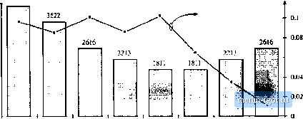

0.06

25 Шг 50кНг 1ГОкНг 200 kHz 25UkHz 400 kHi 500 tHz 1000 кНг Switching frequency

Fig. 15,7 Variation of transformer size (bar chart) with switching frequency, Cuk converter example. Optimum peak ac liux density (data points) is also plotted.

It is a worthwhile exercise to repeat the above design at several different switching frequencies, to determine how transforiner size varies with switching frequency. As the switching frequency is increased, the core k)ss coefficient K increases. Figure 15.7 illustrates the transformer pot core size, for various switching frequencies over the range 25 kHz to 1 MHz, for this Cuk converter example using P material with P,, < 0.25 W. Peak flux densities in Tesla are also plotted. For switching frequencies below 250 kHz, increasing the frequency causes the core size to decrease. This occurs because of the decTeased applied volt-seconds \. Over this range, the optimal Ай is essentially independent of switching frequency; the AB variations shown occur owing to quantization of core sizes,

For switching frequencies greater than 250 kHz, increasing frequency causes greatly increased core loss. Maintaining < 0.25 W then requires that AB be reduced, and hence the core size is increased. The minimum transformer size for this example is apparently obtained at 250 kHz.

In practice, several matters complicate the dependence of transformer size on switching frequency. Figure 15,7 ignores the winding geometty and copper losses due to winding eddy currents. Greater power losses can be allowed in larger cores. Use of a different core material may alioW higher or lower switching frequencies. The same core material, used in a different application with different specifications, may lead to a different optimal frequency. Nonetheless, examples have been reported in the literature [1] in which ferrite transformer size is minimized at frequencies ranging from several hundred kilohertz to several megahertz. More detailed design optimizations can be performed using computer optimization programs [5, Й].

15.3.2 Example 2: Multiple-Output Full-Bridge Buck Converter

As a second example, let us consider the design of transformer Tj for the multiple-output full-bridge buck converter of Fig. 15.8. This converter has a 5 V and a 15 V output, with maximum loads as shown. The transformer is to be optimized at the full-load operating point shown, corresponding to D = 0.75. Waveforms are illustrated in Fig. 15.9, The converter switching frequency is /j = 150 кНг. In the full-bridge configuration, the transformer waveforms have fundamental frequency equal to one-half of the switching frequency, so the effective transformer frequency is 75 kHz. Upon accounting for losses