Fig. 17.18 Notching of ilie ac line-line voltage wavefortiiii dtiring the commutation iilteivals.

essentially only the powei system soutce itnpedance, then cotnmutation causes significant notching of the ac voltage waveforms (Fig. 17.18) at the point of common coupling of the rectifier to the power system. Other elements connected locally to the power system will experience voltage distortion. Limits for the areas of these notches are suggested in lEEE/AKSI standard 519.

17.4

HARMONIC TRAP FILTERS

Passive filters ate often etnployed to reduce the current harmonics generated by rectifiers, such that harmonic limits are met. The filter network is designed to pass the fundamental and to attenuate the significant harmonics such as the fifth, seventh, and perhaps several higher-order odd nontriplen harmonics. Such filters are constructed using resonant tiink circuits tuned to the harmonic frequencies. These networks ate most commonly employed in balanced three-phase systems. A schematic diagram of one phase of the filter is given in Fig. 17.19.

The ac power system is nnodeled by the thevenin-equivalent network containing voltage source and impedance Z/. Impedance Z, is usually inductive in nature, although resonances may occur due to nearby power-factor-correction capacitors. In most filter networks, a series inductor/-/ is employed; the filter is then called a harmonic trap filter. For purposes of analysis, the series inductor /./ can he lumped intoZ as follows:

zд.v)=z;(.v)-лL;

(17.12)

TTie rectifier and its current harmonics are modeled by current source i. Shunt impedances Z Z,... are

ac source tnodel

Harmonic traps (series resotiata networks}

Rectifier model

Fig. 17.19 A harmonic trap filter One phase is illustrated, mi a line-to-neutral basis.

bm&d such that they have low impedance at the harmonic frequencies, and hence the harmonic currents tend to flow through the shunt impedances ratherthan into the ac power system.

The approxiinate algebra-on-the-graph method described in Chapter 8 is used here to construct the filter transfer function, in terras of impedance Z, and the shunt itnpedances Zj, Zj ... This approach yields a simple intuitive understanding of how the filter operates. Since the harmonic frequencies are close in value, the pole and zero frequencies ofthe filter are never well separated in value. So the approximate algebra-on-the-graph method is, in general, not sufficiently accurate for the complete design of these filters, and the pole frequencies must be found by numerical methods. A typical design approach might involve estimating element values using the algebra-on-the-graph method, then refining the values using a computer simulation package.

The filter transfer function H{s} is given by the current divider ratio

His)

Z, + ZJZj...

As discussed in Chapter 8, another way to write this transfer function is

(17.13)

(17.14)

So we can construct H{s) by first constructing the parallel combination Z, Zj Zj then dividing by the total line impedance Z. It can be shown that, ifZ(i) contains no poles, then the numerator of f/(.v) is the product of the zeroes of the shunt impedances Z, So this graphical method yields the exact

zeroes of H{s), which coincide with the series resonances of the shunt impedances. But the poles of His), which arise from parallel resonances in the filter, require more work to compute.

Let us first consider the simple case illustrated in Fig. 17.20, where Zj consists of a series resonant circuit tuned to eliminate the fifth harmonic, and Z, is composed of a single inductor L. Construction of the impedance of a series resonant network is described in Chapter 8. The 1 Z, Ц asymptotes follow the capacitor impedance magnitude 1/шС, at low frequency, and the inductor impedance magnitude COlj at high frequency. At the resonant frequency, ! Zj is equal to The asymptotes for Zj are constructed in Fig. 17.21 (a).

Figure 17.21 (a) also illustrates the impedance magnitude i - as well as construction of

I-00 0 1-

Fig. 17,Z( Simple harmonic trap niter example, containing a series resonant trap tuned to the fifth harmonic, and inductive line impedance.

Fifih-hanrwnic trap Zj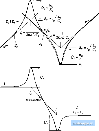

Fig. 17.21 Consiruetlon of approximaie frequency response using the algebra-on-the-graph method: (a) impedance asymptotes, (b) ttansfer fimction asymptotes H .

the approximate asymptotes for the parallel combination(Z, [[ Z). Recall that, to construct the approximate asymptotes for the parallel combination, we simply select the smaller of the and Zj asymptotes. The result is the shaded set of asymptotes shown in the figure: the parallel combination follows ISiL at low frequency, and Ц \\ at high frequency. Note that, in addition to the intended series resonance at frequency/;, a parallel resonance occurs at frequency..

The filter transfer function Я() is now constructed using Eq. (17.14). As illnstrated in Fig. 17.21(b), II H{s) II = 1 at low frequencies where both the numerator and the denominator of Eq. (17.14) are equal to (di,. The parallel resonance at frequency, leads to resonant poles and peaking m Jj H{s) . The resonance at frequency/j leads to resonant zeroes and attenuation in H{s) jj. At high frequency, the gain is LliL + L).

So if we want to attenuate fifth harmonic currents, we should choose the element values such that the series resonant frequency / coiiicide.s with the fifth hai tnonic frequency. This frequency is sim-