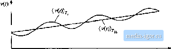Fig. 18,3U Kemovul of coiupoiienls of v(i) at the harmonics of the ac Une freqjcticy, by averaging over one-half ol the ac title period, T.

The output p[)wei is cotnpiised of a constant term v\ , and a term that varies at the secend har-

monic of the ac line Iteqtiency. ТЬе.че two terms are explicitly identified in Fig. 18.29(b).

The second-harmonic variation in {p{t))j- leads lo time-varying system equations, and slow variations in v. , ;() lead lo an output voltage spectrum containing components not only at the frequencies present in 1 , Дг), but also at the even harmonics of the ac line frequency and Iheir sidebands, as well as at the .switching frequency and its harmonics iind sidebands. It is desired to tnodel only the h)w-Irequeticy components excited by slow variations in fo f((). the load, and the ac line voltage amplitude

line period

,j j. The even harmonics of lhe ac line frequency can be removed by averaging over one-half of the ac

7. 1 27t л

(18.94)

Hence, we average over the switching period to remove the switching harmonics, and then average again over one-half of the ac line period T, lo remove the even harmonics of the ac line frequency. The resulting model is valid for frequencies sufficienlly less than the ac line frequency 0). Averaging of the rectifier output voltage is illustrated in Fig. 18.Э0: averaging over Tj reinove.4 the ac line frequency harmonics, leaving the underlying low-frequency variations. By averaging the model of Fig. 18.29(b) over Tjj, we obtain the model of Fig. 18.29(c). This step removes the second-harmonic variation in lhe power source.

The equivalent ciicuit of Fig. 18.29(c) is time-inviuiant, but nonlinear. We can now perturb and linearize as usual, lo construct a small-signal ac model lhal de.scribes how slow variations in v,. i(t), snas rectifier output waveforms. Let us assume that the averaged output vollage

(v(())j., rectifier averaged output current (iit)}, tins line voltage amplitude v, j, and control voltage lJ j,j, ,j(f), can be represented as quiescent values plus sinall slow variations:

(v(f)),=KO(0

(18.95)

with

V -i I Щ1) I

(18,96}

In the averaged model of Fig. 18.29(e), {fl))f,i& given by

(18,97)

This equation resembles DCM buck-boost Eq. (11.45), and lineariiaiion proceeds in a similar manner. Expansion ol Eq. (18.97) in a ihree-dimensional Taylor series aboul ihe quiesceni operating point, and elimination of higher-order nonlinear terms, leads to

(1S.58)

where

4 v . V, v .,.

(18,99)

df V,

-.1г V

(18,100)

(18.101)

A small-signal equivalent circuit based un Eq. (18.98) is given in Fig. 18.29(d). Expressions for the parameters jj, jj, and for several conlruilers are listed in Table 1H. 1. This model is valid Ifn- the conditions ofEq. (18.96), with the additional asstimption that the output voltage ripple is sufliciently small. Figure 18.29(d> is useful only for determining the various ac transfer functions; no information regarding dc conditions can be inferred. The ac resistance is derived from the slope olthe average value olthe power sotirce ouiput characteristic, evaluated at the quiescent operating point. The other coefficients, and g, are also derived from the slopes of the same characteristic, taken with respect to v,j, ,(f) ;ind v and evaluated al the quiescent operating point. The resistance R is the incremental resistance ofthe load, evaluated at the quiescent operating point. In the boost converter with hysteretic control, the transistor on-time ton replaces v.jj ,; as the control inpul; likewise, the iransistor duty cycle d is laken as the

ЪЫе 18.1 Small-signal model parameters for several types of rectilier contiul schemes

Controller type

Average cnrrent control with feedforward. Fig. 18.14

Cunent-programmed control, lf Fig. 18.16

fOrtlineaг-carтier charge control

Of boost rectifier, Fig. 18.21 VV,

Boos: with critical cotiduciion mode 2/

control. Fig. 18.20 vv;;;;;;

DCM buck-boost, flyback, SEPIC, 2P

or Cuk convertert V V.

vv:.

2f VD

control inpul to the DCM buck-boost, Ilyback, SEPIC, and Cuk converters. Harmonics are ignored for the ctirrent-programmed and NLC controllers; the expressions given in Table 18.1 assume that the converter operates in CCM with negligible harmonics. The control-to-outputtransferfunclionis

ад

(18.102)

The line-to-otitput transfer function is

(18.103)

Thus, the small-signal transfer functions of lhe high quality recliliercontain a single pole, ascribable to the outpui lilter capacitor operating in conjunction with the incremental load resistance Д and Tj, the effective output resistance of the power source. Although this model is based on the ideal rectifier, its fonn is similar to that of the dc-dc DCM buck-boo.st converter ac model of Chapter 11. This is natural, because the DCM btick-boost converter is itself a nattiral loss-free resistor. The major difference is that the rms valtie of the ac input vollage musl be used, and lhat the second harmonic components of f*2>J2< and §2 must additionally be removed via averaging. Nonetheless, the equivalent circuit and ac transfer functions are of similar form.

When the rectifier drives a regulated dc-dc converler as in Fig. 18.25, llien the dc-dc converter presents a constant power load to the rectifier, as illustraled in Fig. 18.26. In equilibrittm, tlie rectifier and dc-dc ctmverter operate with the siune average power / , and lhe same dc voltage V. The incremental resistance R of the constant power load is negative, and is given by

R = -

(18.104)

which is equal in magnitude but opposite in polarity to the rectifier incremental output resistance

all conlroliers except the NLC controller. Tlte parallel combination рЦЛ then tends to an open circuit,

and the control-to-output and line-to-otitput transfer Itinclions become