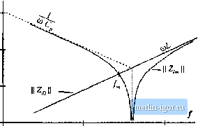Kig. 19.33 Tank network, parallel icsoimnt ooiiratei example: (a) tank eirtiiit, (b) [lode plot Ы input impedance tnagnitude Z for llie limiUiig ciise.4 ff 0 and ff .

(19,45)

As described previously, obtaining good liglit-load efficiency requires tliat II Z,-(/a),} [[ increase as the load resistance R increases. To understand how Zj(juJ,) ]( depends on R, let us sketch ZfjiH) \\ in the extreme cases of an open-circuited {R -* =) andshort-citcuited {R 0) load:

>д.(М)= z,(M)L

z,.(jui.,)=z,(M)

(19.46)

For example, consider the parallel resonant converter ofFigs. 19.19 tt) 19.23. The Bode dia-gratns of the impedatices \\ ZjoCjtiJj and ZJjit)) \\ are constructed in Fig. !9,33. Z,()(j) is found with the load R shorted, and is equal to the inductor impedance sL. Z-Js), found with the load R open-circuited, is given by the seties combination {sL+ \/sC). It can be seen in Fig. 19.33 that the impedance magnitudes Z;[j(;fD,) and II Z; (j(uj) [ intersect at frequency/ . If the switching frequency is chosen such that/, then ZJjO)) \\ > \\ ZOw) , The cotiverter then exhibits the desirable characteristic that the no-load switch current tnagnitude II f,.(/W,) /1 Zj (/u),) i.s stnaller than the switch current under short-circuit conditions, v(J<i}J \\ / \\ Z(J(Oj \\. In fact, the short-circuit switch current is limited by the impedance of the tank inductor, while the open-circuit switch current is determined primarily by the impedance of the tank capacitor.

If the switching frequency is cht)sen such that/,. >/ , then II Z-JJmJ < [ ZiiJiaJ\\. The no-load switch eitrrent is then greater in magnitude than the switch current wheti the load is short-circuited! When the load current is reduced or removed, the transistors will continue to conduct large currents and generate high conduction losses. This causes the efficiency at light load to be poor. It can be concluded that, to obtain good light-load efficiency in the parallel resonant converter, one should choose/, sufficiently less than / . Unfortunately, this requires operation below resonance, leading to reduced output voltage dynamic range and a tendency to lose the zero-voltage switching prtrperty.

A remaining question is how [j Zfjdi) \{ behaves for intermediate values of load between the open-circuit and short-circuit conditions. The answer is given by Theorem 1 below: Z.(yMj j varies monotonically with R. and therefore is bounded by Zjjfjfi),) and ZiJ[j0\} \\ . Hence, the Bode plots of

Series

L C, ШГу-1[-

Pig, 19.34 Series, parallel, and LCC resonant tank networks, and Iheir input iinpetl-ances Z and Zj ,

Parallel L

L C, ЛПЛП-1-

the limiting ea.ses Ц Z.(jCii) {[ and [ Zj(ju)j.) [{ provide a correct qualitative understanding of tlie behavior of ll Zfll for all R. The theorem is valid for lossless tank networks.

Theorem 1; If the tanlt networlt is purely reactive, tlien its input impedance Z. is a monotonic function of tlie load resistance R.

This theorem is proven by use of IVIiddiebrooks Extra Element Theorem (see Appendix C). The tanlt network input impedance Zs) can he expressed as a function ofthe load resistance R and the tank network driving-point impedances, as foiioWS:

Zfs} = Z (s)

Z,J.s)

AM

(19,47)

where Z- and Zf are the resonant network input impedances, with the load short-circuited or open-circuited, respectively, and Zand Z, are the resonant network output impedances, with the source input short-circuited or open-circuited, respectively. These terminal impedances are simple functions ofthe tank elements, and their Bode diagrams are easily constructed. The input impedances ofthe series reso-

iiiiiit, piinillel resonant, and LCC inverters are listed in Fig. 1У.34. Sinee these impedances do not depend on the load, they ate purely reactive, ideally have zero real parts [38], and their complex conjugates are given hy = - Z, - - Z, etc. Again, recall that the tnagnittide of a complex impedance Z(ja>) can he expressed as the square root of Z(jlii)Z(J(ii). Hence, the tnagnitude of Zj(.i) is given hy

1 +

7.Js)

1 +

(19.48)

vt-here Z is the complex conjugate of Zj,

Next, let us differentiate Eq. (19.48) with respect to R:

ll 2R\7 f

1 + -

(19.49)

The derivative has roots at (i) R - 0, (ii) Й = = , and in the special case (иг) where Zf, = Z. . Since the derivative is otherwise nonzero, the resonant network input impedance Z; is a nionotonic ftinction of R, over the range 0 < Л < oo. in special case ( /), Z; is independent of R. Therefore, Theorem 1 is proved.

An example is given in Figs. 19.3f> and 19.35, for the LCC inverter. Figure 19.35 illustrates the impedance asymptotes of the limiting cases Zj,j and Zjj, . Variation of Zj between these limits, forfmite nonzero Л, is illustrated in Fig. 19.36. The open-circuit resonant frequency and the short-circuit resonant frequency/, are given by

(19.50)

where СЦdenotes inverse addition of Cjand C:

C.fC,= 1

(19.51)

For the LCC inverter, the impedance magnitudes Z;y and Z- \\. are equal at frequency/, given by

2k7LCJ2C