Fig. 7.10 Use of the average slope to ptedict how the inductor current waveform changes over one . 1гсИ!П5 period. The actual waveform ((() and its low-frequency componeitt (ifr)) are illustrated.

Actual vfaveforrn. Averaged waveform including tipple

d{v,u)),d{m),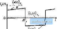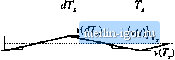

(vw).. Шг. mr,

RC RC с

Fig. 7,11 Buck-boost converter wavefonns: (a) tfap.icitor current, (b) capacitor voltage.

removed. Also, the use of the average slope leads to correct prediction of the final value It can be easily verified that, when Eq. (7.23) is inserted into Eq, (7.19), the previous result (7.14) is obtained.

7.2.3 Averaging the Capacitur Wavefurms

A similar procedure leads to the capacitor dynamic equation. The capacitor voltage and current wave-f[)rms are sketched in Fig. 7.11. The average capacitor current can be found by averaging Eqs. (7.8) and (7.12); the result is

+d\t)

(7.24)

Upon inserting this equation into Eq. (7.2) and collecting terms, one obtains

7.2 TTie Bunic A С Modeling Appmack

(7.23)

Ibis is the basic averaged equation which describes dc and low-frequency ac variations in the capacitor voltage.

7.2.4 The AvertigE Input Current

In Chapter 3, it was foimd to be necessary to write an additional equation that models the dc component ofthe converter input current. This allowed the inputport of the converter to be modeled by the dc equivalent circuit. A similar procedure must be followed here, so that low-frequency variations at the converter input port are modeled by the ac equivalent circuit.

For the buck-boost converter example, the Current iU) drawn by the COtlverter from the input .source is equal lo the inductor current i(f) during the Titbit subinterval, and zero during the second sub-interval. By neglecting the inductor current ripple and replacing i(f) with its averaged value OCO),. we can express the input current as follows:

(i(/))j. during subinterval 1 {) during subinterval 2

(7.26)

The input current waveform is illustrated in Fig. 7.12. Upon averaging over one switching period, one oblains

(7.27)

This is the basic averaged equation which describes dc and Itjw-frequency ac variations in the converter input ctirrent.

7.2.S PerturbtitJon and LinearizatJon

The buck-boost converter averaged equations, Eqs. (7.14), (7.25), and (7.27), are collected below:

L-J-I

These equations are nonlinear because they involve the multiplitation of time-varying quantities. For example, the tapaeitor current depends on the produet of the eontrol input ifU) and the low-frequency component of the inductor current, (ttf))?;- Multiplicatton nf time-varying signals generates harmonics, and is a tionltnear process. Most of the techniques of ac circuit analysis, such as the Laplace transform and other frequency-domain methods, are not useful for nonlinear systems. So we need to linearize Eqs. (7.2S) by constructing a small-signal model.

Suppose that we drive the converter at some steady-state, or quiescent, duty ratio d{t) = D, with quiescent input voltage f,(0 = V. We know froin our steady-state analysts of Chapters 1 and 3 that, after any transrents have subsided, the inductor current {t(f)),, the capacttor voltage (у{1)), and the input current {ijpbr, will reach the quiescent values /, V, and l, respectively, where

(7.29)

Equations (7.29) are derived as usual via the principles of inductor volt-second atid capacitor charge balance. They could also be derived froin Eqs. (7.28) by noting that, in steady state, the derivatives inust equal zero.

To construct a small-signal ac model at a quiescent operating point (/, V), one assumes that the input voltage v{t) and the duty cycle d{!) are equal to soine given quiescent values V, and D. plus some superimposed small ac variations v{t) and (/(r). Hetice, \ve have

In response to these inputs, and after atiy transients have subsided, the averaged inductor current (i(/))j., the averaged capacitor voltage (i());;. and the averaged input cunent {,(0); waveforms will be equal to the corresponding quiescent values /. V, and plus some superimposed small ac variations i(l)., v{t), and

{t(r)),=/+((/)

(v(()) = V+v{() (7.31)

(,(0)=/,(/)

With the assumptions that the ac variations arc small in magnitude compared to the dc quiescent values,