DKi)

!dU)C) С Ф v(() к R

Fig. 7.14 Circuit equivaleni to the sntall-signiil ac ciipiicitiiriiode eciualinn of Bq, (7,43) or (7,39).

0 >©

Fig. 7,1S Circuil etiiiivaieilt to lire small-signal i\c input sotirce ctirreitt etpiatiou of Eq, (7,43) or (7,42),

ognized as the current flowing through the load resi.stor in the .small-.signal model. The resistor is connected in parallel with the capacitor, such that the ac voltage across the resistor R is v(f) as expected. The term Щ{) is driven by the control iiiputf/(0, and is represented by an independent source as shown.

Finally, the input current equation of (7.43), or Eq. (7,42), describes the small-signal ac current l(f) drawn by the converter out of the input voltage source P.O)- This is a node equation which states that i(t) is equal to the currents in two branches, as illustrated in Fig. 7.15, The first branch, corresponding to the ОГ{01егп1, is dependent tm the ac inductor current t(i). Hence, we represent this term using a dependent current source; this .source will eventually be incorporated into an ideal transformer. The second branch, corresponding to the ii?(i) term, is driven by the control input J(/), aud is represented by an independent source as shown.

The circuits of Figs. 7.13, 7.14, and 7.15 are collected in Fig. 7.1fi(a). As discussed in Chapter 3, the dependent sources can be combined into effective ideal transformers, as illustrated in Fig. 7.16(b). The sinusoid superimposed on the transformer symbol indicates that the transfurmer is ideal, and is part of the averaged small-signal ac model. So the effective dc transformer property of CCM dc-dc converters also influences small-signal ac variations in the conveiter signals.

The equivalent circuit of Fig. 7.1(i(b) can now be solved using techniques of conventional linear circuit analysis, to find the converter transfer functions, input and output impedances, etc. This is done in detail in the next chapter. Also, the model can be refined by inclusion of losses aud other nonidealities- an example is given in Section 7.2.9.

7.2.7 Discussion of the Perturbation and Linearization filep

In the perturbation and linearization step, it is assumed that an averaged voltage or current consists of a constant (dc) component and a small-signal ac variation around the dc component. In Section 7.2.5, the

oo,<o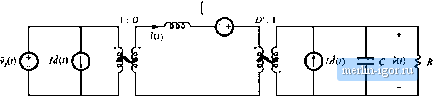

Fig, 7,16 Buclc-bousl cnnverter smiill-bignal ac equivalent circjit: (a) the circnits of bigs. 7.13 to 7.15, collected logeEher; (b) combination iif dcpendoit sources into effective tdeid tiansfortner, leading li> the final ]iiodel.

linearization step wa.s completed by neglecting nonlinear Eerins that correspond to products of the small-signal ac variations. In general, the linearization step amounts to talting the Taylor expansion of a nonlinear relation and retaining only the constant and linear terms. For example, the large-signal averaged equation for the inductor current in Eq. (7.28) can be written as:

(7.44)

Let ufi expand this expression in a three-dimensional Taylor series, about the quiescent operating point (V, V.Dy.

[dt dt j

V = V

d(t)

v= v

+ liigher-order iionlinear terms

(7.45)

For simplicity of notation, the angle brackets denoting average values are dropped in the above equation. The derivative of / is zero, since i is by defiiution a dc (constant) term. Equating the dc terms on both sides of Eq, (7.45) gives:

(7,46)

which is the volt-second balance relationship for the inductor. The coefficients with the linear terms on the right-hand side of Eq. (7.45) are found as follows:

(7,47)

v = V

d = D

= V,.-K

(7.49)

Using (7.47), (7,48) and (7,49), neglecting higher-order nonlinear terras, and equating the linear ac terms on both sides of Eq. (7.45) gives:

L = Dv(f) + Df(0 + [ V, - V) M

(7.50)

which is identical to Eq. (7.36) derived in Section 7.2.5. In conclusion, the linearization step can always be accomplished using the Taylor expansion.

7.2.S Results for Several Basic Converters

The equivalent circuit models for the buck, boost, and buck-boost converters operating in the continuous conduction raode arc suramarized in Fig. 7.17. The buck and boost converter models contain ideal transformers having turns ratios equal to the converter conversion ratio. The buck-boost converter contains ideal transformers having buck and boost conversion ratios; this is consistent with the derivation of Section 6.1.2 of the buck-boost converter as a cascade connection of buck and bcKist converters. These models can be solved to find the converter transfer functions, input and output impedances, inductor current variations, etc. By insertion of appropriate turns ratios, the equivalent circuits of Fig. 7.17 can be adapted to model the transforraer-isolated versions of the buck, boost, and buck-boost converters, including the forward, tlyback, and other converters.

7.2.9 Example: A Nonideal Flyback Converter

To illustrate that the techniques of the previous section are useful for modeling a variety of converter phenoraena, let us next derive a small-signal ac equivalent circuit of a converter containing transformer isolation and resistive losses. An isolated flyback converter is illustrated in Fig, 7.IS, The flyback transformer has magnetizing inductance L, referred to the primnry winding, and turns ratio 1 \iu MOSFET has on-resistance R, . Other loss elements, as well as the transformer leakage inductances and the switching losses, are negligible. The ac modeling of this converter begins in a manner similar to the dc converter analysis of Section 6.3,4. The flyback transformer is replaced by an equivalent circuit consisting of the magnetizing inductance L in parallel with an ideal transformer, as illustrated in Fig. 7.19(a).

During the fust subinterval, when MOSFET conducts, diode is off. Tlie circuit then