7.1 Tht Easic AC Modeling Approach

Fig. 7,23 Circuit Mjuivalent to tlic smaLI-sigiiitl ac indtictor lotip equatitm, Eq. (7.76) or

(7,66).

Dv,(r)

ЛЛг

d{t)[v~]R., +l

-it-

We neglect the second-ortler nonlinear tertns of Eq, (7.72), leaving the following linearized ac equation:

j\(/) = Ui{t) + lim (7-74)

This result models the low-frequency ac variations in the converter input current.

The equations of the quiescent values, Eqs, (7.65), (7.69), and (7.73) are collected below:

a = DV-D-DRJ

л R

(7.75)

C = D/

For given quiescent values ofthe input voltage and duty cycle D, this system of equations can be evaluated to find the quiescent output voltage V, indtictor current 7, and input current dc component/. The results are then inserted into the small-signal ac equations.

The small-signal ac equations, Eqs. (7.66), (7.70), and (7.74), are summarized below:

dkt) d,

= DvU) - U! + [ + ]f - d(l) - DRj{()

, dm Oi(r) C(r) idtjX dl Я

(7.76)

The final step is to construct an equivalent circuit that corresponds to these equations.

The inductor equation was derived by first writing loop equations, to find the applied iitductor voltage during each subinterval. These equations were then averaged, perturbed, and linearized, to obtain Eq. (7.66), So this equation describes the small-signal ac voltages around a Кюр containing the inductor. The loop current is the ac inductor current t(f). The quantity Ldiiiydt is the low-frequency ac voltage acToss the inductor. The four terms on the right-hand side ofthe equation are the voltages across the four other elements in the loop. The terms Ovt) and - DviiVn are dependent on voltages elsewhere in the converter, and hence iue represented as dependent sources in Fig. 7.23. The third terra is driven by the duty cycle variations d(f)and hence is represented as an independent source. The fourth term, - DRJ(t), is a voltage that is proportional tt) the k)op current i(t). Hence this term obeys Ohms law, with effective resistance OR as shown in the figure. So the influence ofthe MOSFET on-resistance on the converter

ТЛПГ

mi dt

ACEqiiivalm! Circwl Modeling

Fig. 7.24 Circuit equivalent to the small-signal ac capacitor node equation, Eq, (7.76) or (7,70).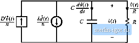

Fig. 7,15 Circuit equivalent to the small-signal ac input source current equation, Eq. (7.76) or (7.74).

snrall-signal transfer functions is modeled by an effective resistance ofvalue D/f .

Sniall-sigiial capacitor equation (7.70) leads to the equivalent circuit of Fig. 7.24. The equation constitutes a node equation of the equivalent circuit model. It states that the capacitor current Cdv{tydth equal to three other currents. The current Diif)/n depends on a current elsewhere in the mtKlel, and hence is represented by a dependent current source. The term - vii)/R is the ac component of the load current, which we model with a load resistance Я connected in parallel with the capacitor. The last temi is driven by the duty cycle variations d{t), and is modeled by an independent source.

The input port equation, Eq. (7.74), also constitutes a node equation. It describes the small-signal ac current 10, drawn by the converter out of the input voltage source 0((). There are two other terms in the equation. The term Di{i) is dependent on the inductor current ac variation t(/), and is represented with a dependent sotirce. The term ld(t) is driven by the control variations, and is modeled by an independent source. The equivident ciicuit for the input port is illustrated in Fig. 7.25.

The circuits of Figs. 7.23, 7.24, and 7.25 are combined in Fig. 7.26. The dependent soiu-ces can be replaced by ideal transformers, leading to the equivaleni circuit of Fig. 7.27. This is the desired result: an equivalent circuit that models the low-frequency small-signal variations in the converter waveforms. It can now be solved, using conventional linear circuit analysis techniques, to find the converter transfer functions, outptit impedance, and other ac quantities of interest.

tfS)

i*(0

-Лг-

DP, )

4 C)!M с Ф HO l

Fig, 7.2Й The oquivaletu circuits of Figs. 7.23 lo 7.2S, collected togedier.

1 :D

OD:n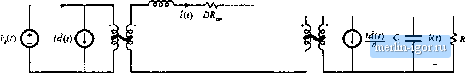

Hg> 7.27 Smali-signal ac equivalent circuit model of the flyback converter.

STATE-SPACE AVERA(;iN(;

A number of ac converter modeling techniques have appealed in the literature, including the current-injected approach, circuit averaging, and the state-space averaging method. .Although the proponents of a given method may prefer to express the end result in a specific form, the end results of nearly all methods lire equivalent. And everybody will agree that averaging and sinall-signal linearization are the key steps in modeling PWM converters.

The state-space averaging approach [1,2] is described in this section. The state-.чрасс description of dynamical systems is a mainstay of intHlem control theory; the state-space averaging methtxl niiikes use of this description to derive the small-signal averaged equatioits of PWM switching convertei. The state-space averaging methtxl is otherwise identical to the procedure derived in Section 7.2, Indeed, the procedure of Section 7.2 amounts to state-space averaging, but without the formality of writing the equatitms in matrix form. A benefit ofthe state-space averaging procedure is the generality of its result: a small-signal averaged mtxiel can always be t>btaiiied, provided that the state equations of the original convertercan be written.

Section 7.3.1 summarizes how to write the state equations of a network. The basic results of state-space averaging are described in Section 7.3.2, and a short derivation is given in Section 7.3.3. Section 7.3.4 contains an example, in which the state-space averaging method is used to derive the quiescent dc ;md small-signal ac equations of a buck-boost converter.

7.3.1 The State Equations of a Network

The state-space description is a canonical form for writing die differential equations that describe a system. For a lineiu network, the derivatives of the stale variables are expressed as linear combinations of the system independent inputs and the state viuiables themselves. The physical state variables of a system are usually associated with the storage of energy, and for a typical converter circuit, the physical state variables are the independent inductor currents and capacitor vtdtages. Other typical state variables include the position and velocity of a motor shaft. At a given point in time, the values ofthe state variables depend on the previous history of the system, rather than on the present values ofthe system inputs. To solve the differential equations of the system, the initial values ofthe state viuiables must be specified. So if we know the state of a system, that is, the values trf all ofthe state variables, at a given time tg, and if we additionally know the system inputs, then we can in principle st>lve the system state equatitms to find the system waveforms at any future time.

The state equations of a system can be written in the compact matrix form of Eq. (7.77):