y(0 = CK(f) + Fu(()

(7.77)

Here, tlie state vector x(/) is a vector containing ali of tlie state variables, that is, the inductor currents, capacitor voitages, etc. The input vector u(f) contains the independent inputs to the system, such as the input voltage source vjt). The derivative of the state vector is a vector whose elements are equal to the derivatives of the conesponding elements of the statB vector:

x(0 =

fi() x,(.t]

dxU) lit

dx,{t)

<lt

dx,{t)

(7,7K)

In the standard form ofEq. (7.77), К is a matrix containing the values of capacitance, inductance, and mtitual inductance (if any), such that Kdx(iydl is a vector containing the indtictor winding voltages and capacitor currents. In other physical systems, К may contain other qtiantities such as moment of inertia or mass. Equation (7.77) states that the inductor voltages and capacitor currents of the system can he expressed as linear combinations of the state variables and the independent inputs. The matrices A and В contain constants of proportionality.

It may also be desired to compute other circuit waveforms that do not coincide with the elements of the state vector x(f) or the input vector u(r]. These other signals are, in general, dependent waveforms that can he expressed as linear combinations of the elements of the state vector and input vector. The vector y(f) is usually called the output vector. We are free to place any dependent signal in this vector, regardless of whether the signal is actually a physical otitput. The converter input current i(t) is often chosen to be an element ofy(f). In the state equations (7.77), the elements of y(r) are expressed as a linear combination of the elements of the x(f) and u(r) vectors. The matrices С and E contain constants of proportionality.

As an example, let tis write the state equations of the circuit of Fig. 7,28. This circuit contains two capacitors and an inductor, and hence the physical state variables are the independent capacitor voltages Vj(() and vit), as well as the inductor current l(t). So we can define the state vector as

X(f) =

Vi(t)

(7.79)

Fig. 7.28 Circuit example.

Since there are no coupled inductors, the matrix К is diagonal, and simply contains the values of capacitance and inductance:

Ci 0 0

0 [)

0 0 L

(7,80)

The circuit has one independent input, the current source /,- (0. Hence we should define the input vector as

(7.81)

We are free to place any dependent signal in vector )>(/). Suppose that we are interested in also computing the voltage /0 and the current We can therefore define y(f) as

y(t) =

(7.82)

To write the state equations in the canonical form of Eq. С1.П), we need to express the inductor voltages and capacitor currents as linear combinations of the elements of x(f) and u(f), that is, as linear combina-tioits of V(/), v,(/), 1(0, and ; (/).

The capacitor current i((0 is given by the node eqtiation

W,) = C, = UO--*)

(7.83)

This equation will be>come the top row of the matrix, equation (7.77). Tlie capacitor current (r) is given by the node equation.

(7.84)

Note that we have been careful to express this current as a linear combination of the elements of x(f) and u(/) alone. The inductor voltage is given by the loop eqtiation.

MO = /- = Vi(n-v,(0 Equations (7.83) to (7.85) can be written in the following matrix form:

(7.85)

C, 0 0

0 Cj 0 0 0 L

-tL о

3 + к,

v,(0

(7.86)

\(t) + В u(r)

Matrioe.4 A aud В are ntiw known.

It i.s also neces.sary to express the elemeiit.s ot y(() as linear comhinations of the eletnents of x(;) and u(r). By solution of the eircuit of Fig. 7.28, v, (t) can he written in terms of v(t) as

(7,87)

Also, fflj(Ocan he expressed in terms of fifOas

V,(f)

(7.88)

By collecting Eqs. (7.87) and (7.S8) into the standard matrix form ofEq. (7.77), we obtain

y(t) =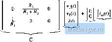

(7,89)

m + E ait)

We can now identify the matrices С and E as shown above.

It should be recognized that, starting in Chapter 2, we have always begun fhc analysis of converters by writing their state equations. We are now .simply writing these equations in matrix form.

7.3.2 The Basic State-Space Averaged Model

Consider now that we are given a PWM converter, operating in the continuous conduction mode. The converter circuit contains independent states that fonn the state vecttw xU), and the ctmverteris driven by independent sources that form the input vector u(f). During the first subintcrvai, when the switches are in position 1, the converter reduces to a linear circuit that can be described by the following state equations:

K = AiS(/) + B,u(/) y(f) = C,x(/) + E,u(()

(790)

During the second subinterval, with the switches in position 2, the converter reduces to another linear circuit whose state equations are

K = AjXCOBiU(/) y(f) = CjJt(() + EiU(()

(7.91)

During the two subintervals, the circuit elements are connected differently; therefore, the respective state equation matrices Aj, ilj, Cj, К, and Aj, B, C, Щ may also differ. Given these state equations, the result of state-space averaging is the state equations of the equilibrium and sinaii-signai ac models.

Provided that the natural frequencies of the converter, as well as the frequencies of variations of the converter inputs, are much slower than the switching frequency, then the state-space averaged model