result is

{y{t))j =(/(0fc,{x(l))r +E,(u(0)] + rfi;t)(Cj(x(t)) 1-E,{ (0) \ (7.107)

Rearrangement of terra.s yields

This is again a nonlinear equation.

The averaged state equations, (7,106) and (7.108), are oolleeted below:

d{i) A. + dV) A,] (51(0)+ [dit) В, + d(t) Bj] {11(f))

{m)r{m c, + d\t) Ci) {x(o)j./((J(OE,+d(t) Ej) (uo)).,.

(7.108)

(7Л09)

The next step is the linearization of these equations about a quiescent operating point, to construct a small-signal ac model. When dc inputs d(t) = D and u(() = U are applied, converter operates in equilibrium when the derivatives of all of the elements of {х(/)} are zero. Hence, by setting the derivative of (x(f))jj to zero in Eq. (7.109), we can define the converter quiescent operating point as the solution of

0=AX+BU Y = CX + RU

(7.110)

where definitions (7.93) and (7.94) have been used. We now perturb and linearize the converter waveforms about this quiescent operating point:

(s(0)r=X.Hi(O (ii(0)=U + O(0

d{t) = D + d(r) d\t) = a-S(,t)

(7.111)

Here, U(() and d{t) are small ac variations in the input vector and duty ratio. The vectors x(0 and y(f) are the resulting small ac variations in the state and output vectors. We must assume that these ac variations are much smaller than the quiescent values. In other words.

Xls.K(0 111-*№)

Here, к X ii denotes a norm of the vector x.

Substitution DfEq. (7.11 1) into Eq. (7.109) yields

(7.112)

ri(X+ S(f))

Л+ d(l}]A , 4 (D-(/(f)] Л J (X+ (f)) D-K/(o)Bi + (D-d(/))lij (u+0(f))

+ [D+dU)]E, + {Ly--thn]E, [U+u(0) The derivative dX/rfr is zero. By eoUecting terras, one obtains

КхЩ = (aX + BU]+\S<t) + Ba(f) + [A,-Aj)X + (Bi-B3)uy(/)

first-order EC dc terms first-order ac (ernrs

+ (a 1 - A i)x(r)i(0 + (Bi - Bi)a(f)

second-order nonlinear terras

(7,113)

(7,114)

{Y*m] = (CX + EUj + cm + Kfl(0 + {[C,- C,)X - (e, -E,)uy(f)

dc + 1 order ac de terms first-order ae terms

+ (C, - Сз)х(/)J(f) + (E, - Ej]u(/V(t) v,

second-order nonlinear terms

Sinte the dt terms satisfy Eq. (7.110), they drop ont of Eq. (7.114). Also, if the stnali-signal assumption (7.112) is satisfied, then the second-order nonlinear terms of Eq. (7.114) are small in magnitude compared to the first-order ac terms. We can therefore neglect the nonlinear terms, to obtain the following linearized ac model:

. ffS(0 dt

y(() = Cx(/)-(-Efl(/) +

К = Ax(() -r m/} + (A, - A i] X + (в, - в J uU(f)

(C,-C,)X + (E,-E,] Vthi)

(7.115)

This is the desired result, which coincides with Eq. (7.95).

7.3.4 Example: State-Space Averaging uf a Nonideal Buck-Boost Converter

Let lis apply the state-space averaging methtxl to model the buck-btx)st converter of Fig. 7.31. We will model the conduction loss of MOSFET byon-resistance Л , and the forward voltage drop of diode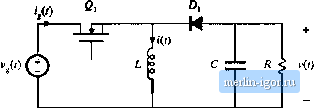

Fig, 7,31 Cuck-boost converter example.

i>] by an independent voltage source ofvalue V. It is desired to obtain a complete equivalent circuit, which models both the input port and the output port of the converter,

The independent states of the converter ate the inductor current ;{/) and the capacitor voltage \>(f). Therefore, we should define the state vector x(r) as

\{!}--

v(!)

(7.116)

The input voltage vU) is an independent source which should be placed in the input vector u(r). hi addition, we have chosen to model the diode forward voltage drop with an independent voltage source of value Vq. So this voltage source should also be included m the input vector ii(r). Therefore, let us define the input vector as

u(f) =

(7.117)

To model the converter input port, we need to rind the converter input current ((;). To calculate this dependent current, it should be included in the output vector y(r). Therefore, let us choose to define y{l) as

y(r) =

i,il)

(7.118)

Note that it isnt necessary to include the output voltage v{t] in the output vector y((), since v{t) is already included in the state vector x(r).

Next, let us write the state equations for each subinterval. When the switch is in position 1, the converter circuit of Fig. 7.32(a) is obtained. The inductor voltage, capacitor current, aud converter input current ate

/. = v (0-i(O/t,

clvit) v(()

(7,119)

dt ~ R

i,it) = Hl)

These equations can be written in the following state-space form: