Fig, S,6 Magnitude asymptotes for itie single real pole transfer fimetion.

!GOto)jB J

-20 dB -

-60 dB

-20 dB/decade

C(>tu))-OdB

Thus, as illustrated in Fig. 8.6. at low frequency G(/ai) is asymptotic to 0 dB. At high frequency, м (й atid /э/о. In this case, it is true that

;& 1

We can then say that

(8.20)

(M.21)

Hetice, Eq. (8.15) m)w becomes

G(jto)=-

(8,22)

This expression coincides with Eq. (8.5), with n = -1. So at high frequency, й(/(й) has slop -20 dB per decade, as illustrated in Fig. 8.6. Thus, the asymptotes of G(/0)) are equal to 1 at low frequency, and ( f,) at high frequency. The asymptotes intersect at /(]. The actual magnitude tends toward these asymptotes at very low frequency and very high frequency. In the vicinity ofthe corner frequency/ц, the actual curve deviates somewhat from the a.4yinptotcs.

The deviation of the exact curve from the asymptotes can be found by simply evaluating Eq. (8.15). At the corner frequency /=/.Etj. (8.15) becomes

C(M)1 =

In decibels, the magnitude is

f.-(M>

= -3dB

(8,23)

(8,24)

So the actual curve deviates from the asymptotes by -3 dB at the corner frequency, as illustrated in Fig. 8.7. Similar arguments show that the actual curve deviates from the asymptotes by -1 dB at /=/ц/2

IGOco)[,B j

Kig. 8.7 Deviation of tlie actual curve from the asymptotes, real pole.

-tOdB -

-ZOdB

-30 dB

-20 dB/decade

and at /= 2/).

The phase of G(j(u) is

RefoOtu))

ZCa) = tan

Insertion of the re;il and imaginary parts ofEq. (8.14) into Eq. (8.25) leads to

ZG(.;(i3) = - tun

(8.25)

(8.26

This function is plotted in Fig. 8.8. It tends to 0° at low frequency, and to -90° at high frequency. Atthe corner frequency /=/(), the phase is -45.

Since the high-frequency and low-frequency phase asymptotes do not intersect, we need a third asymptote to approximate the phase in the vicinity of the comer frequency /).One way to do this is illus-

0 asymptote

Fig. 8,8 Exact phase plot, single real pale.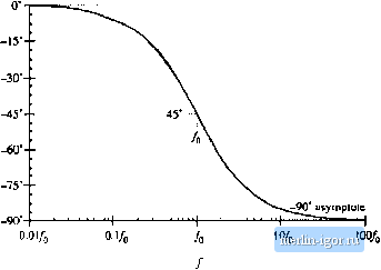

Kg. 8.9 One choice for the mid frequency phase asymptote, which correctly predicts the actual slupe at/=/ .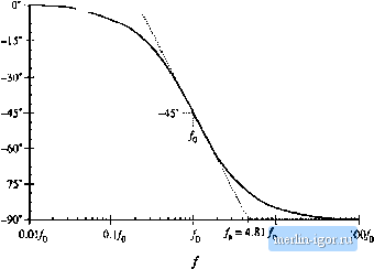

tiated in Fig. where the slope of the asymptote is chosen to be identical to the slope of the actual curve at/ = /(у It can be shown that, with this choice, the asymptote intersection frequencies and /j, are given by

(8,27)

A simpler choice, which better approximates the actual curve, is

- -to

(Й.2Й)

This asymptote is compared to the actual curve in Fig. 8.10. The pole causes the phase to change over a frequency span of approximately two decades, centered at the corner frequency. The slope ofthe asymptote in this frequency span is -45 per decade. At the brealc frequencies and the actual phase deviates from the asymptotes by tan~(0.1) = 5.7°,

The magnitude and phase asymptotes for the single-pole response arc summarized in Fig, 8.11.

It is good practice to consistently express single-pole transferfunctions in the normalized form of Eq. (8,12). Both terms in the denominator of Eq. (8.12) are dimensionless, and the coefficient of is unity. Equation (8.12) is easy to interpret, because of its normalized form. At low frequencies, where the (iViOo) term is small in magnitude, the transfer function is approximately equal to 1. At high frequencies, where the (i/tUj,) tenn has magnitude much greater than 1, the transfer function is approximately (.t/u)[,). This leads to a magnitude of (P/[,). The corner frequency is = (Oln. So the transfer function is written directly in terms of its salient features, that is, its asymptotes and its corner frequency.