Qmvfrrer Тгапфг Functions

For example, eonsider constmetion of the Bode plot of the following tratisfer funetion:

1+ш7

(8,45)

where Gj, = 40

32 db./ = t0/27t = 100 Hz,/j = (i)j/27l = 2 kHz. Thistransfer function contains three terms: the gain Gq, and the poles at frequencies yjand /-The asymptotes for each of these terms are illustrated in Fig. 8.16. The gain Gq is a positive real number, and therefore contributes zero pha.se shift with the gain 32 dB. The poles at 1(Ю Hz and 2 kHz each contribute asymptotes as in Fig. 8.11.

At frequencies less than ]tX) Hz, the G term contributes a gain magnitude of 32 dB, while the two pt)les each contribute magnitude asymptotes of 0 dB. So the low-frequency composite magnitude asymptote is 32 dB + 0 dB + 0 dB = 32 dB. For frequencies between 1Ю Hz and 2 kHz, the Cngain again contributes 32 dB, and the pole at 2 kHz continues to contribute a 0 dB magnitude asymptote. However, the pole at 100 Hz now contributes a magnitude asymptote that decreases with a -20 dB per decade slope. The composite magnitude asymptote therefore alst) decreases with a -20 dB per decade sk)pe, as illustrated in Fig. 8.16. For frequencies greater than 2 kHz, the pt)les at 1(X) Hz and 2 kHz each contribute decreasing asymptotes having slopes of -20 dB/decade. The composite asymptote therefore decreases with a slope of-20 dB/decade -20 dB/decade = 0 dB/decade, as illustrated.

The composite phase asymptote is also constructed in Fig. 8.16. Below 10 Hz, all terms contribute 0° asymptotes. For frequencies between = 10 Hz, and /jlO = 200 Hz, the pole atcontributes a decreasing phase asymptote having a .slope of-457decade. Between 2(X) Hz and 10/, - 1 kHz, both poles contribute decreasing asymptotes with -45/decade slopes; the composite slope is therefore -907decade. Between 1 kHz and IO/2 = 20 kHz, the pole at/[ contributes a constant -90° phase asymptote, while the pole at/j contributes a decieirsing asymptote with -457decade slope. The composite slope is then ~45°/decade. For frequencies greater than 20 kHz, both poles contribute constant -W asymptotes, leading to a ctmipt)site phase asymptote of-180°.

As a second example, consider the transfer function A{s) rep- II II resented by the magnitude and

phase asymptotes of Fig. 8.17. Let

us write the transfer function that corresponds to these asymptotes. The dc asymptote is Ац. At comer frequency /, the asymptote slope increases from 0 dB/decade to +20 dB/decade. Hence, diere must be a zero at frequency /,. At frequency /j, the asymptote slope decreases from +20 dB/decade to 0 dB/ decade. Therefore the transfer function contains a pole at frequency/j. So we can express the transfer function as

+20 dB/decade

+4i7dec

JVdecade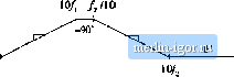

/,/10

Fig, 8.17 Magnitude aud phase asymptotes of example transfer function Л (л).

a(j) = a

1 + r

(8.46)

where and Cuj are equal to 2л.f and 271/3, respectively.

We can use Eq. (S.46) to derive analytical expressions for the asymptotes. For/</, and letting s = we can see that the (j/ojj) and (.t/cOj) terms each have inaguitude less than 1. The asyinptote is derived by neglecting these terms. Hence, the low-frequency magnitude asymptote is

(8.47)

For / <f<fi. thenumerator term (i/u))has magnitude greater than 1, while the denominator terra (j/ro) has magnitude less than 1. The asymptote is derived by neglecting the smaller terms:

-A - 4 2

(B.48)

This is the expression for the midfiequenty magnitude asymptote oiA(s). For/>/2, the (.v/tOj) and (siijif) terms each have magnitude greater than 1. The expression for the high-frequency asyinptote is therefore:

(S.49)

S= 1<M

We can conclude that the high-frequency gniti is

(ii.50)

Thus, we can derive analytical expressions for the asymptotes.

The transfer function AU) can also be written in a second form, using invetled poles and zeroes. Suppose that A{s) represents the transfer function of a high-frequency amplifier, wht)se dc gain is not important. We are then interested in expressing Л(.!) directly in terms ofthe high-frequency gain A . We can view the transfer function as having an inverted pole at frequency/2, which introduces attenuation at frequencies less than/j. In addition, there is an inverted zero slf=fy So Л(.?) could also be written

A(s)=A.

(8.51)

h can be verified that Eqs. (8.51) and (8.46) are equivalent.

8.1.6 Quudrutic Pole Response: Resonance

Consider next tiie transfer function Gis) of the two-pole low-pass filter of Fig. 8. IS. The buck converter contains у a filter of this type. When manipulated into canonical form, the models of the boost and buck-boost also contain similar filters. One can show that the transfer function of this network is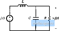

Fig. 8.18 Two-poie low-pass filter example,

(8.52)

This transfer function contains a second-order denominator polynomial, and is of the form

G(s) =

1 +a,s + flj.s-

(S.53)

with й =L/f;and j = LC.

To construct the Bode plot of this transfer function, we might try to factor the denominator into its two roots:

G{s) =

-:)(-t)

Use of the quadratic formula leads to the following expressions for the roots:

1-,/ 1-

4(1,

(8.54)

(8.55)

/, 4

(8.56)

If 2 - l hen the roots are real. Each real pole then exhibits a Bode diagram as derived in Section 8.1.1, and the ct)mposite Bode diagram can be constructed as described in Section 8.1.5 (but a better approach is described in Section S.l.7).

If4a2 5 /Д then the roots (8.55) and (8.56) are complex. In Section 8.1.1, the assumption wm made that fflo is real; hence, the results of that section cannot be applied to this case. We need to do some additional work, to determine the magnitude and phase for the case when the roots are complex.

The transfer functions of Eqs. (8.52) and (8.53) can be written in the following standard normalized form:

(8.57)

If thecoefficients and 2 are real and positive, then the parameters Q and are also real and positive. The parameter Шц is again the angular corner frequency, and we can definetil(/2jt. The parameter is