called the damping factor. controls the shape t)f the transfer function in the vicinity of/ = /q. An altei-native standard normalized form is

where

(8.5S)

(8,59)

The parameter Q is called the quality factor of the circuit, and is a ineasure of the dissipation in the system. A more general definition of Q, for sinusoidal excitation of a passive element or network, is

Q = ln

(peak stoiedeneigy) (energy dissipated per cycle)

(8 60)

For a second-order passive system, Eqs. (8.59) and (8.60) are equivalent. We will .see that the Q-i-Actoi has a very simple interpretation in the magnitude Bode diagrams of second-order transfer functions.

Analytical expressions for the parameters Q and ti) can he found by equating like powers of.? in the original tiansfer function, Eq. (8.52), and in the normalized form, Eq. (8.58). The result is

11 . 1 ° 2n 211/LC

(8.61)

The lOOts .t, and of Eqs. (8.55) and (8.56) ;ire real when Q < 0,5, and are complex when Q > 0.5. The magnitude of G is

II ajiJi) II - -

Asymptotes of Ц G \\ are illustrated in Fig. 8.19. At low frequencies, (u)/Uy) 1, and hence

IIСII -> 1 for to <K (D

(8.62)

(8.ЙЗ)

-+t) (IB

-60 dB

o.i/o Л

Fig, S.li> Magnitude asymptotes tor the two-pole transfer function.

lO/o

At high frequencies where a;. 1, the (tu/Ct) ) term

(iominates the expression inside the radical of Eq. (8.62). Hence, the high-frequency asymptote is

tor tl):

(8.64)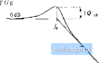

0 dB/decade

This expression coincides with Eq. (8.5), with jt = -2. Therefore, the high-frequency asymptote has slope -40 dB/

decade. The asymptotes intersect at/= L, and are indepen- ,. j.

, ff-f J f Fig. 8.20 Important teatures of the magni-

dent ot Q. jjjj jjyj pjjjj ijij. t,.p,lg u-ansfer

The parameter Q affects the deviation of the actual function curve frt)m the asymptotes, in the neighborht)od t)f the corner frequency , The exact magnitude at/=/) is found by substitution of W = Ь) into Eq. (8.62):

So the exact transfer function has magnitude Q at the corner frequency/,. In decibels, Eq. (8.65) is

llwl,.=lc?. t

So if, for example, Q = 2 =3i 6 dB, then the actual curve deviates from the asymptotes by 6 dB at the corner frequency/=./q. Salient features of the magnitude Bode plot of the second-order transfer function are summarized in Fig, 8,20, The phase of G is

ZGijo:} = tan

Q I

(8.67)

The phase tends to 0 at low frequency, and to -180° at high frequency. At/ = /( the phase is-90 . As illustrated in Fig, 8.21, increasing the value of Q causes a sharper phase change between the 0 and -180° asymptotes. We again need a midfrequency asymptote, to approximate the phase transition in the

Increasirtg Q

Ffe. 8,21 Ptiase plot, sccoiid4)rdor poles. Increasing Q causes a sharper phase change.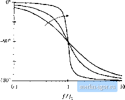

Fig. 8.22 One choice Ibr the iTiidtVeciteiicy phase asymptote of the two-pole response, which correctly predicts the actual slope at

-90=--

-180

Fig. Й.13 A simpler choice for the niidfrequeney phase asyinptote, wtiich better approjtimate.4 the curti over the entire frequency range and is consistent with the asymptote used for real poles.

-90°--

-180

vicinity of the comer frequency fy, as illustrated in Fig. 8.22. As in the ca.se of the real single pt)le. we ctndd chtjose the slope of this asymptote to be identical to the slope of the actual curve а/=У. It can be shown that this choice leads to the following asymptote break frequencies: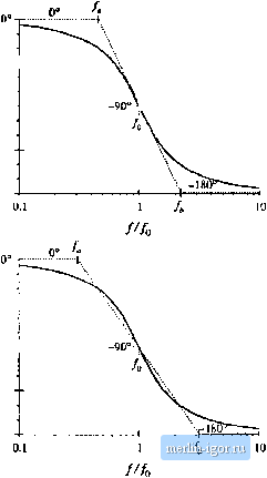

A better choice, which is consistent with the approximation (8.28) used for the real single pole, is

/,= 10- Vu

(8.68)

(3.69)

With this choice, the midfrequency asymptote has slope -180 degrees per decade. The phase asymptotes are summarized in Fig. 8.23. With Q - 0.5, the phase changes from 0° to -180° over a frequency span of approximately two decades, centered at the corner frequency /q. Increasing the Q causes this frequency span to decrease rapidly.

Second-Older response magnitude and phase curves are plotted in Figs. 8.24 and 8.25.