Fig, 8.14 Gxiicl imgnitudc ciiivsa, wo-pole lesponse, for sevcriil values otQ.

10 dB

-lOdB

-20 dB

Fig. 8.2S hxucl phase ULirves, [wn-pole response, for several values of Q.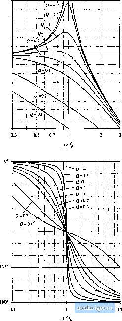

S.1.7 The Lmv-Q Appru\imatioit

As mentioned in Section 8.1.6, when tlie toots of second-order denominator polynomial of Bq. (8.53) are real, then we can factor the denominator, and construct the Bode diagram using the asymptotes for real poles. We would then и.че the following normalized form:

This is a particularly desirable approach when the comer frequencies tUj and cu are well separated in value.

The difficulty in this procedure lies in the complexity ofthe quadratic formula used to find the corner frequencies. Expressing the comer frequencies (0, aud (U in terras t)f the circuit elements fi. L, С etc., invariably leads to complicated and unillurainating expressitras, especially when the circuit contains many elements. Even in the case of the simple circuit of Fig. 8.18, whose transfer function is given by Eq. (8.52), the conventional tiuadratic formula leads to the following complicated formula for the corner frequencies:

o) o),= --

-iLC (8,71)

This equation yields essentially no insight regarding how the corner frequencies depend on the element values. For exaraple, it can be shown that when the comer frequencies itre well separated in value, they can be expressed with high accuracy by the much simpler relations

0 L (ii.72)

El this case, (Uj is essentially independent ofthe value of C, and fflj is essentially independent of L, yet Eq. (8.71) apparently predicts that both corner frequencies are dependent on all element values. The simple expressions of Eq. (8.72) are far preferable to Eq. (8.71), and can be easily derived using the low- approximation [2].

Let us assume that the transfer function has been expressed in the standard normalized form of Eq. (8.58), reproduced below:

For Q< 0.5, let us use the quadratic formula to write the real roots ofthe denominator polynomial of Eq. (8.73) as

M l-v/t-4CJ (8.74)

Q 2

1 + у I - 4Q (8,75)

Fig. 8.26 F{Q) vs. as givcci by Eq, (8.77). The ujtijroiimattoii F(Q) = I is within \Ш of the exact value for G < 3.

The corner frequency CO can be expressed

0.75 - -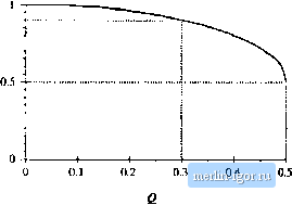

0.25 - -

(8.76)

where F(Q) is defined as [2]:

F(0) = (l+\Te

Note that, when Q 0.5, then 4Q -V- 1 and F{Q) is approximately equal to 1. We then obtain

to, = forC?

(8.77)

(8.78)

The function F{Q) is plotted in Fig. 8.26. It can be seen that F{Q) approaches 1 very rapidly as Q decreases below 0.5.

To derive a similar approximation lor we can multiply and divide Eq. (8.74) by F(Q\ Eq. (8.77). Upon simplification of the numerator, we obtain

F(Q)

(8,79)

Again, F{Q) tends to 1 for small Q. Hence, со, can be approximated as

u), Qjifi for Q 2

(8.80)

Magnitude asymptotes for the low-g са.че are summarized in Fig, 8.27. For Q < 0.5, the two poles at (Uo split into real poles. One real pole occurs at corner frequency to <{i)g, while the other occurs at corner frequency tO > ю,. The corner frequencies are easily approximated, using Eqs. (8.78) and (8.80).

For the filter circuit of Fig. 8.18, the paratneters Q and (О are given by Eq. (8.61). For the ca.se when Q 0,5, we can derive the following analytical expressions for the corner frequencies, using Eqs. (8.78) and (8.80):