Fig. 8,37 Magnitude asympwtcs predicted by the lriw-(2 approximaiion, Real poles occur at frequencies Qf aad ffQ.

-Ай dB/decaffi

LC jf fC

fLC 1 1

(8,81)

So the low-й approximation allows us to derive simple design-oriented analytical expressions for the corner frequencies.

8.1.S Approxiitifite Roots of an Arbitrary-Degree Polynomial

The low-й approximation can be generalized, to find approximate analytical expressions for the rottts of the n*-order polynomial

It is desired to factor the polynomial P{s) into the form

P[j)=[l + T,.f)(l-bT,;s)-(l + vj

(8.82)

(8,83)

In a real circuit, the coefficients л a are real, while the time constants Tj,.... t may be either real or complex. Very often, some or ail of the time constants arc well separated in value, and depend in a very simple way on the circuit element values. In such cases, simple approximate analytical expressions for the time constants can be derived.

The time constants T,.....can be related to the original coefficients a a,j by multiplying

out Eq. (8.83). The result is

(8,84)

General solution of this system of equations amounts to exact factoring of the arbitrary degree polynomial, a hopeless task. Nonetheless, Eq. (8.84) does suggest a way to approximate the roots.

Suppose that all ofthe time constants Tj, T,are real and well separated in value. We can further assume, without loss of generality, that the time constants are arranged in decreasing order of magni-

tude:

T, T,

When the inequalities ofBq. (B.85) are satisfied, then the expressions ford . dominated by their first terms:

a, -T,

These expressions can now be solved for the time constants, with the result

(8,65)

, rt of Eq. (8.84) are each (8.86)

(8.87)

Hence, if

then the polynomial P{s} given hy Eq. (8.82) has the approximate factorization F(s) = (l+a,]

(8.88)

(8.89)

Note that if the original coefficients in Eq. (8.82) are simple functions of the circuit elements, then the approximate roots given hy Eq. (8.89) are similar simple functions of the circuit elements. So approximate analytical expressions for the roots can he obtained. Numerical values are substituted into Eq. (8.88) to justify the approximation.

In the ciise where two of the roots же not well separated, then one of the inequalities of Eq. (8.88) is violated. We can then leave the corresponding terms in quadratic form. For example, suppose that inequidity к is not satisfied:

(8.У0)

Then an approximate factorization is

s.l Revieve of Bode PloK

II CL = 20106,(1 СII The conditions for accuracy of this approximation are

(8,91)

(8.92)

Complex conjugate roots can be approximated in this manner.

When the first ineqtiality of Eq. (8.88) is violated, that is.

then the first two roots should be left in quadratic form

This approximation is justified provided that

(8.93)

(8.94)

(8.95)

If none of the above approximations isjustified, then there are three or more roots that are close in magnitude. One must then resort to cubic or higher-order forms.

As an example, consider the damped EMI filter illustrated in Fig. 8,28. Filters such as this are typically placed at the power Input of a converter, to attenuate the switching harmonics present in the converter input current. By circuit analysis, on can show that this filter exhibits the following transfer function:

V(J) Gis) = f- =

This transfer function contains a third-order denominator, with the following coefficients:

(8.96)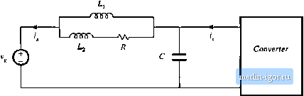

Fig. 8.28 input EM I filter example.