(8.97)

It is desired to factor tlte deuoininator, to obtain analytical expressions for the poles. The correct way to do this depends on the numerical values qIR,L, L, and C. When the roots are real and well separated, then Eq. (8.89) predicts that the denominator can be factored as follows:

1 +s

\+sRC

According to Eq. (8.88), this approximation isjustified provided that

(8,98)

(8,99

Ttiese inequalities cannot be satisfied unless L. When L, l, then Eq. (8.99) can be further simplified to

(ii.iOO)

The approximate factorization, Eq. (8.98), can then be further simplified to

Thus, in this case the transfer function contains three well separated real poles. Equations (8.98) and (8.101) represent approximate analytical factorizations of the denominator of Eq. (8.96). Although numerical values tnust be substituted into Eqs. (8.99) or (8.100) to justify the approximation, we can nonetheless express Eqs. (8.98) and (8.101) as analytical functions of L L, R. and C. Equations (8.98) and (8.101) are design-oriented, because they yield insight into how the element values can be chosen such that given specified pole frequencies are obtained.

When the second inequality ofEq. (8.99) is violated.

Л, + Z,2 R

then the second and third roots should be left in quadratic form:

(8.i02)

(8,10.4)

This expression follows from Eq. (8.91), with к = 2. Equation (8.92) predicts that this approximation is justified provided that

S.2 Analysis of Convener Transfer Functions

(8.104)

In application t)f Eq. (8.92), we talte а to be equal to 1. The inequalities of Eq. (8.104) can be siinplifietl to obtain

Л,.1;. and RC

(8.105)

Note that it is no longer required that RC Lj/ff, Equation (8.105) implies that factorization (8.103) can he further simplified to

1 +i-

1 + jfiC + .v=L,C

(3.106)

Thus, lor this case, the transfer function contains a low-frequency pole that is well separated from a high-frequency quadratic pole pair. Again, the factored result (8.106) is expressed as an analytical function of the element values, and consequently is design-oriented.

Iti the ca.se where the first inequality of Eq. (8.99) is violated:

then the first and second roots should be left in quadratic form:

(S.107)

(8.108)

This expression follows directly from Eq. (8.94). Equation (8.95) predicts that this approximation isjustified provided that

that is.

f.,fiC f.,+J f., J.J R R

f.,3-L and RC

(8.109)

(a.ilo)

For this case, the transfer function contains a low-frequency quadratic pole pair that is well separated from a high-frequency real pole. If none of the above approximations are justified, then all three of the roots are similar in magnitude. We must then find other means of dealing with the original cubic polyno-tnial. Etesign of input filter.s, including the filter of Fig. 8.28. is ctwered in Chapter 10.

ANALYSIS OF CONVERTER TRANSFER FUNCTIONS

Let u.4 next derive analytical expressitms for the poles, zeroes, and asympt[)te gains in the transfer functions of the basic ctmverters.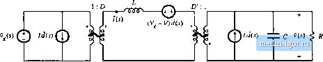

Fig. Я.29 Hut к-boost cotiverter equivalent circuit derived in .Section 7.2.

8.2.1 Example: Transfer Functions of the Buck-Boost Converter

The small-sigual equivalent circuit model of the buck-boost converter is derived in Section 7.2, with tlie result [Fig. 7.16(b)] repeated in Fig. 8.29. Let us derive and plot the control-to-output and line-to-output transfer functions for tliis circuit.

The converter contains two independent ac inputs: the contr[)l input and the line input f,(l The ac output voltage variations iis) can be expressed as the superposition of terms arising from these two inputs:

C(:) = GJs)J{s) + C;, (j) v.v) Hence, the transfer functions 0,s} and OJ,s) can be defined as

ад . , v(s)

and G,Js)=

(h.lll)

(8. II2)

rt.)-ii

To find the line-to-output transfer function G,J\), we .set the il sources to zero as in Fig. 8.30(a). We can then push the vja) .source and the inductor through the transformers, to obtain the circuit of Fig. 8.30(b). The transfer function C;,,(i} is found using the voltage divider formula:

1 -.D

D: ]

С V{5) < R

Fig, Я.,3в Manipulation of btick-boost cquivaieitt c\rcm to find f!ie linc-fo-OHtpUl tratwfei fuiicdoit Gis): (it) set d sources to y.em; (b) pn.4li tntliictor and source dirotigh tiansfomicr.