8.2 Analysis of Convener Transfer Funaions 295

(8.113)

We next expand the parallel et)tnbinati[)ii, and exptess as a rational fraetion:

R \

\*.;RC}

i-D] R

1 +sfiC

(8.114}

We arent done yet-the next step is to manipulate the expression into nortnalized form, suoh that the coefficients of s in the numerator and denominator polynomials are equal to one. This can be accotn-plished by dividing the nuraeratorand denominator by R:

R D

(8.iI5)

Thus, the line-to-output transfer function contains a dc gain Ciq and a quadratic ptile pair:

(8.116)

Analytical expressions for the salient features ofthe line-to-output transfer function are fotmd by equating like tenns in Eqs. (8.115) and (8.11Й). The dt gain is

By equating the coefficients of i in the detioniinators of Eqs. (8.115) and (8.116), we obtain

(8.П7)

(8.118)

Hence, the angidar comer frequency is

By equating coefficients of.? in the denotninators of Eqs. (8.115) and (8.116), we obtain

1 L Q(u lyR

(8.119)

(8.120)

Elimination of using Eq. (8.119) and solution for Q leads to

Convener Тгапфг Fmiaions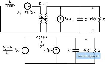

Fig. 8.31 Manipulaiion of buck-boost etiiiivalciit circuit to find thi; control-to-output transfer function G,j(j): (a) set v, source to zero; (b) push inductor and voltage source through transformer

{8.121)

Equations (8.117), (8.119), and (8.121) are the desired results in the analysis of the line-to-output transfer function. These expressitms are useful not only in analysis situations, where it is desired to find numerical values of the salient features iiQ, Щ, and Q, but also in design situations, where il is desired to select numerical values for/t, L and С such that given values of the salient features are obtained.

Derivation of the control-to-output transferfunction Cv,/) is complicated by the presence in Fig. 8.29 of three generators that depend on One good way to find Gj(.v)is to manipulate the circuit model as in the derivation of the cantjnical model. Fig. 7.60. Atiother approitch, used here, employs the principle of superposition. First, we set the v, source to zero. This shorts the inptit to the 1:D transformer, and we are left with the circuit illustrated in Fig. 8.31(a). Next, we push the inductor and d voltage source through the D:l transformer, as in Fig. 8.3 i(b).

Figure 8.31(b) contains a (/-dependent voltage source and a -dependent current s[)urce. The transfer fimction G,(i) can therefore be expressed as a supeфosition of terms arising from these two sources. When the current source is set to zero (i.e., open-circuited), the circuit of Fig. 8.32(a) is obtained. The output v(s) can then be expressed as

(8.i22)

When the voltage source is set to zero (i.e., short-circuited), Fig. 8.31(b) reduces to the circuit illustrated in Fig. 8,32(b). The output i(.v) can then be expressed as

dis) ~

(8,123)

The transferfimction Gfs) is the sum of Eqs. (8.122) and (8.123):

s.2 Aimlysi.i of Converter Transfer Fwiclioiis 297

Fig. 8.32 Solution of the model of Fig. 8.32(b) by superposition: (a) current source set to zero; (b) voltage source set to zero.

о cdp m к R

v,-v

rL

(?,124)

By algebraic tnanipulation, one can reduce this expression to

(8.125)

This equation is ofthe form

(8.126)

Tliedentminators ofEq. (8.125) atid (8.115) ate identical, and hence Gi) andGj,(jJshare the aametilfl and Q. given by Eqs. (8.119) and (8.121). The dc gain is

V - V V,

s V

(8.127)

The angular frequency of the zero is found by equating coefficients of .5 in the numerators of Eqs. (8.125) and (8.126). One obtains

LI DL

(RHP)

(3.128)

This zero lies in the right half-plane. Equations (8.127) and (8.128) have been simplified by use ofthedc relationships