8.2. THE TURING MACHINE 317

and system designer than do the undecidable problems. The reason is that, while undecidable problems are usually quite obviously so, and their solutions are rarely attempted in practice, the intractable problems are faced every day. Moreover, they often yield to small modifications in the requirements or to heuristic solutions. Thus, the designer is faced quite frequently with having to decide whether or not a problem is in the intractable class, and what to do about it, if so.

We need tools that will allow us to prove everyday questions undecidable or intractable. The technology introduced m Section 8.1 is useful for questions that deal with programs, but it does not translate easily to problems in unrelated domains. For example, we would have great difEicidty reducing the hello-world problem to the question of whether a grammar is ambiguous.

As a result, we need to rebuild our theory of undecidability, based not on programs in С or another language, but based on a very simple model of a computer, called the Turing machine. This device is essentially a finite automaton that has a single tape of infinite length on which it may read and write data. One advantage of the Turing machine over programs as representation of what can be computed is that the Turing machine is sufficiently simple that we can represent its configuration precisely, using a simple notation much like the IDs of a PDA. In comparison, while С programs have a state, involving all the variables in whatever sequence of function calls have been made, the notation for describing these states is far too complex to allow us to make understandable, formal proofs.

Using the Turing machine notation, we shall prove undecidable certain problems that appear unrelated to programming. For instance, we shall show in Section 9.4 that Posts Correspondence Problem, a simple question involving two fists of strings, is undecidable, and this problem makes it easy to show questions about grammars, such as ambiguity, to be undecidable. Likewise, when we introduce intractable problems we shall find that certain questions, Seemingly having little to do with computation (e.g., satisfiability of boolean formulas), are intractable.

8.2.1 The Quest to Decide All Mathematical Questions

At the turn of the 20th century, the mathematician D. Hilbert asked whether it was possible to find an algorithm for determining the truth or falsehood of any mathematical proposition. In particular, he asked if there was a way to determine whether any formula in the first-order predicate calculus, applied to integers, was true. Since the first-order predicate calculus of integers is sufficiently powerful to express statements like this grammar is ambiguous, or this program prints hello, world, had Hilbert been successful, these problems would have algorithms that we now know do not exist.

However, in 1931, K, Godel published his famous incompleteness theorem. He constructed a formula in the predicate calculus applied to integers, which asserted that the formula itself could be neither proved nor disproved within

the predicate calculus. Godels technique resembles the construction of the self-contradictory program H2 in Section 8.1.2, but deals with functions on the integers, rather than with С programs.

The predicate calculus was not the only notion that mathematicians had for any possible computation. In fact predicate calculus, being declarative rather than computational, had to compete with a variety of notations, including the partial-recursive functions, a rather programming-language-like notation, and other similar notations. In 1936, A. M. Turing proposed the Turing machine as a model of any possible computation. This model is computer-like, rather than program-like, even though true electronic, or even electromechanical computers were several years in the future (and Turing himself was involved in the construction of such a machine during World War II).

Interestingly, all the serious proposals for a model of computation have the same power; that is, they compute the same functions or recognize the same languages. The unprovable assumption that any general way to compute wUl allow us to compute only the partial-recursive functions (or equivalently, what Turing machines or modern-day computers can compute) is known as Churchs hypothesis (after the logician A. Church) or the Church-Turing thesis.

8.2.2 Notation for the Turing Machine

We may visualize a Turing machine as in Fig. 8.8. The machine consists of a finite control, which can be in any of a finite set of states. There is a tape divided into squares or cells; each cell can hold any one of a finite number of sjTnbols.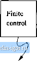

Figure 8.8: A Turing machine

Initially, the input, which is a finite-length string of symbols chosen from the input alphabet, is placed on the tape. All other tape cells, extending infinitely to the left and right, initially hold a special symbol called the blank. The Ыгшк is a tape symbol, but not an input symbol, and there may be other tape symbols besides the input symbols and the blank, as well.

There is a tape head that is always positioned at one of the tape cells. The Turing machine is said to be scanning that cell. Initially, the tape head is at

the leftmost cell that holds the input.

A move of the Turing machine is a function of the state of the finite control and the tape symbol scanned. In one move, the Turing machine will:

1. Change state. The next state optionally may be the same as the current state.

2. Write a tape symbol in the cell scanned. This tape symbol replaces whatever symbol was in that cell. Optionally, the symbol written may be the same as the symbol currently there.

3. Move the tape head left or right. In our formalism we requure a move, and do not allow the head to remain statiouEuy. This restriction does not constrain what a Turing machine can compute, since any sequence of moves with a stationary head could be condensed, along with the next tape-head move, into a single state change, a new tape symbol, and a move left or right.

The formal notation we shall use for a Turing machine (TM) is similar to that used for finite automata or PDAs. We describe a TM by the 7-tuple

whose components have the following meanings: Q: The finite set of states of the finite control. S: The finite set of input symbols.

Г: The complete set of tape symbols; S is always a subset of Г.

5: The transition function. The arguments of S{q,X) are a state q and a tape symbol X. The value of 5{q,X), if it is defined, is a triple (p,F, D), where:

1. p is the next state, in Q.

2. У is the symbol, in Г, written in the cell being scanned, replacing whatever symbol was there.

3. Z> is a direction, either L or R, standing for left or right, respectively, and telling us the direction in which the head moves.

qo: The start state, a member of Q, in which the finite control is found initially.

B: The u/oTjfc symbol. This symbol is in Г but not in S; i.e., it is not an input symbol. The blank appears initially in all but the finite number of initial cells that hold input symbols.

F: The set of final or accepting states, a subset of Q.