a) Show how, given a TM that computes /, you can construct a TM that accepts the graph of / as a language.

b) Show how, given a TM that accepts the graph of /, you can construct a TM that computes /.

c) A function is said to be partial if it may be undefined for some arguments. If we extend the ideas of this exercise to partial functions, then we do not require that the TM computing / halts if its input x is one of the integers for which f{x) is not defined. Do your constructions for parts (a) and (b) work if the function / is partial? If not, explain how you could modify the construction to make it work.

Exercise 8.2.5: Consider the Turing machine

M = {{qo, quq2,q!}, {0,1}, {0,1, B},&,qo, B, {qj})

Informally but clearly describe the language i(M) if consists of the following sets of rules:

* a) %o, 0) - {qi, 1, Д); , 1} - (o, 0, R); S{qi, B) = {qf,B, R).

b) 5(90,0) - {qo>B,R); 5{qQ,l) = ((/.,Я,Л); 6{дг,1) - {quB,Ry,5{q B) = {qS,B,R).

c) 5{qo,0) - {qxA,R); 6{q l) - (g2,0,L); 6{q2,l) = {qoA,R); S{qi,B) = {Qf,B,R).

8.3 Programming Techniques for Turing Machines

Our goal is to give you a sense of how a Turing machuie can be used to compute in a manner not unlike that of a conventional computer. Eventually, we want to convince you that a TM is exactly as powerful as a conventional computer. In particular, we shall learn that the Turing machine can perform the sort of calculations on other Turing machines that we saw performed in Section 8.1.2 by a program that examined other programs. This introspective ability of both Turing machines and computer programs is what enables us to prove problems undecidable.

To make the ability of a TM clearer, we shall present a number of examples of how we might think of the tape and finite control of the Turing machine. None of these tricks extend the basic model of the TM; they are only notational conveniences. Later, we shall use them to simulate extended Turing-machine models that have additional features - for instance, more than one tape - by the basic TM model.

8.3.1 Storage in the State

We can use the finite control not only to represent a position in the program of the Turing machine, but to hold a finite amount of data. Figure 8.13 suggests this technique (as well as another idea: multiple tracks). There, we see the finite control consisting of not only a control state q, but three data elements A, B, and C. The technique requires no extension to the TM model; we merely think of the state as a tuple. In the case of Fig. 8.13, we should think of the state as [q, A, B, С]. Regarding states this way allows us to describe transitions in a more systematic way, often making the strategy behind the TM program more transparent.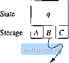

Track 1 Track 2 Track 3

Figure 8.13: A Turing machine viewed as having finite-control storage and multiple tracks

Example 8.6: We shall design a TM

M {Q, {0,1}, {0,1, B}, 6, [qo, B], {[91, B]})

that remembers in its finite control the first symbol (0 or 1) that it sees, and checks that it does not appear elsewhere on its input. Thus, M accepts the language 01*+ 10*. Accepting regular languages such as this one does not stress the ability of Turing machines, but it wiU serve as a simple demonstration.

The set of states Q is {qo,qi} x {0,1, B}, That is, the states may be thought of as pairs with two components:

a) A control portion, go or qi, that remembers what the TM is doing. Control state qo indicates that M has not yet read its first symbol, white gi indicates that it has read the symbol, and is checking that it does not appear elsewhere, by movmg right and hoping to reach a blank cell.

b) A data portion, which remembers the first symbol seen, which must be 0 or 1. The symbol В in this component means that no symbol has been read.

The transition function <J of M is as follows:

1. 6{[qo,B],a) = ([дьа],а,Л) for a = 0 or a - 1. Initially, go is the control state, and the data portion of the state is Б. The symbol scanned is copied into the second component of the state, and M moves right, entering control state gi as it does so.

2. 6{[qi,a\,a) = ([gi, a],a, R) where a is the complement of a, that is, 0 if a - I and 1 if a = 0. In state gi, M skips over each symbol 0 or 1 that is different from the one it has stored in its state, and continues moving right.

3. 6([qi,a],B) = {[qi,B],B,R) for a = 0 or a = 1. If M reaches the first blank, it enters the accepting state [qi,B].

Notice that M has no definition for i[qi,a],a) br a - 0 от a - 1. Thus, if M encounters a second occurrence of the symbol it stored initially in its finite control, it halts without having entered the accepting state. □

8.3.2 Multiple Tracks

Another useful trick is to think of the tape of a Turing machine as composed of several tracks. Each track can hold one symbol, and the tape alphabet of the TM consists of tuples, with one component for each track. Thus, for instance, the cell scanned by the tape head in Fig. 8.13 contains the symbol [АГ,У, Z]. Like the technique of storage in the finite control, using multiple tracks does not extend what the Turing machine can do. It is simply a way to view tape symbols and to imagine that they have a useful structure.

Example 8.7: A common use of multiple tracks is to treat one track as holding the data and a second track as holding a mark. We can check off each symbol as we use it, or we can keep track of a small number of positions within the data by marking only those positions. Examples 8,2 and 8.4 were two instances of this technique, but in neither example did we think explicitly of the tape as if it were composed of tracks. In the present example, we shall use a second track explicitly to recognize the non-context-free language

Lwcw - {wcm I № is in (0 + 1) }

The Turing machine we shall design is:

M = {Q, S, Г, Й, [gi, S], [B,B], {[qs,B]})

where:

Q: The set of states is {i, 92, - i99} x {0,1, Б}, that is, pairs consisting of a control state qi and a data component: 0, 1, or blank. We again use the technique of storage in the finite control, as we allow the state to remember an input symbol 0 or 1.