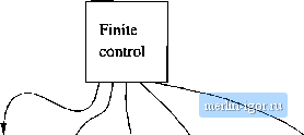Instruction counter

Memory address

Computers Input file

Scratch

И0П10

Figure 8.22: A Turing machine that simulates a typical computer

involved in the computation. First, the desired address is copied onto tape 3 and compared with the addresses on tape 1, until a match is foimd. The contents of this address is copied onto the third tape and moved to wherever it is needed, typically to one of the low-numbered addresses that represent the registers of the computer.

Our TM will simulate the instruction cycle of the computer, as follows.

1. Seaich the first tape for an address that matches the instruction number on tape 2. We start at the $ on the first tape, and move right, comparing each address with the contents of tape 2. The comparison of addresses on the two tapes is easy, since we need only move the tape heads right, in tandem, checking that the symbols scaimed are always the same.

2. When the instruction address is found, examine its value. Let us assume that when a word is an instruction, its first few bits represent the action to be taken (e.g., copy, add, branch), and the remaining bits code an address or addresses that are involved in the action.

3. If the instruction requires the value of some address, then that address will be part of the instruction. Copy that address onto the third tape, and

mark the position of the instruction, using a second track of the first tape (not shown in Fig. 8.22), so we can find otn way back to the instruction, if necessary. Now, search for the memory address on the first tape, and cojiv its value onto tape 3, tlie tape that holds the memory address,

4. Execute the instruction, or the part of the instruction involving this value. Wo cannot go into all the possible machine instructions. However, a sample of the kinds of things we might do with the new value are:

(a) Copy it to some other address. We get the second address from the instnictitm, find this address by putting it on tape 3 and searching for the address on tape 1, as discussed previously. When we find the second address, we copy the value into the space reserved for the value of that address. If more space is needed for the new value, or the new vahie uses less space than the old valu(!. change the available space by shifting over. That is:

i. Copy, onto a scratch tape the entire nonblank tape to the right of where the new value goes.

ii. Write the new value, using the correct amount of space for that value.

iii. Rocopy the scratch tape onto tape; 1. immediately to tiie right of the new value.

As a specijil case, the address may not yet appear on the first tape, because it Iuls not been used by the computer previously. In this case, we find the place on the first tape where it belongs, shift-over t(; make adequate rtjom, and store both the address and the new value there.

(b) Add the value just found to the vahie of some other address. Go back to the instruction to locate the other address, find this address on tape 1, Perform a binary addition of the value of that address and the value stored on tape 3. By scanning the two values from theii right ends, a. TM can perform a ri])ple-carry addition with little difficulty. Should more spai:e be needed for the result, use the shifting-over technique to create space on tape 1.

(c) The instruction is a jump, that is, a directive to take the next instruction from the address that is the value now stored on tape 3. Simply copy tape 3 to tape 2 and begin the instruction cycle again,

-3. After performing the instruction, and determining that the instruction is not a jump, atid 1 to the instruction counter on tape 2 and begin the instruction cycle again.

There are many other details of how the TM simulates a typical computer, We have suggested in Fig, 8.22 a fourth tape holding the simulated input to the

computer, since the computer mnst read its input (the word whose membership ill a language it is testing) from a file. The TM can read from this tape instead.

A scratch tape is also shown. Simulation of some computer instructions might make effective use of a scratch tape or tapes to compute arithmetic operations such as multiplication.

Finally, we assume that the computer makes an output that tells whether or not its input is accepted. To translate this action into terms that the Turing machine can execute, we shall suppose that there is an accept instruction of the computer, perhaps corresponding to a function call by the computer to put yes on an output file. When the TM simulates the execution of this computer instruction, it enters an accepting state of its own and halts.

While the above discussion is far from a complete, formal proof that a TM can simulate a typical computer, it should provide you with enough detail to convince you that a TM is a valid representation for what a computer can do. Thus, in the future, we shall use only the Turing machine as the formal representation of what can be computed by any kind of computing device.

8.6.3 Comparing the Running Times of Computers and Turing Machines

We now must address the issue of running time for the Turing machine that simulates a computer. As we have suggested previously:

The issue of running time is important because we shall use the TM not only to examine the question of what can be computed at all, but what can be computed with enough efficiency that a problems computer-based solution can be used in practice.

The dividing fine between the tractable - that which can be solved efficiently - from the intractable - problems that can be solved, but not fast enough for the solution to be usable - is generally held to be between what can be computed in polynomial time and what requires more than any polynomial running time.

Thus, we need to assure ourselves that if a problem can be solved in polynomial time on a typical computer, then it can be solved in polynomial time by a Turing machine, and conversely. Because of this polynomial equivalence, our conclusions about what a Turing machine can or cannot do with adequate efficiency apply equally well to a computer.

Recall that in Section 8.4.3 we determined that the difference in running time between one-tape and multitape TMs was polynomial - quadratic, in particular. Thus, it is .sufficient to show that anything the computer can do, the multitape T.M described in Section 8.6.2 can do in an amount of time that is polynomial in the amount of time the computer takes. We then know that the same holds for a one-tape TM.