problem is. Thus, we introduce the notion of polynomial-time reductions in the first section.

There is another important distinction between the Idnds of conclusions we drew in the theory of undecidability and those that intractability theory lets us draw. The proofs of undecidability that we gave in Chapter 9 are incontrovertible; they depend on nothing but the definition of a Turing machine <md common mathematics. In contrast, the results on intractable problems that we give here are all predicated on an unproved, but strongly beUeved, assumption, often referred to as the assumption P ф MV.

That is, we assume the class of problems that can be solved by nondeterministic TMs operating in polynomial time includes at least some problems that cannot be solved by deterministic TMs operating in polynomial time (even if we allow a higher degree polynomial for the deterministic TM). There are ht-erally thousands of problems that appear to be in this category, since they can be solved easily by a polynomial time NTM, yet no polynomial-time DTM (or computer program, which is the same thing) is known for their solution. Moreover, an important consequence of intractability theory is that either all these problems have polynomial-time deterministic solutions, which have eluded us for centuries, or none do; i.e., they really require exponential time.

10.1 The Classes V and AfV

hi this section, we introduce the basic concepts of intractability theory; the classes P and A/P of problems solvable in polynomial time by deterministic and nondeterministic TMs, respectively, and the technique of polynomial-time reduction. We also define the notion of NP-completeness, a property that certain problems in MP have; they are at least as hard (to within a polynomial in time) as any problem in MP.

10.1.1 Problems Solvable in Polynomial Time

A Turing machine M is said to be of time complexity T{n) [or to have nmning time T(n) ] if whenever M is given an input ю of length n, M halts after making at most T{n) moves, regardless of whether or not M accepts. This definition applies to any function T(n), such as T{n) - 50n or T[n) - 3 -b 5n*; we shall be interested predominantly in the case where Г(п) is a polynomial in n. We say a language L is in class P if there is some polynomial T{n) such that L = L{M) for some deterministic TM M of time complexity T(n).

10.1.2 An Example: Kruskals Algorithm

You are probably familiar with many problems that have efficient solutions; perhaps you studied some in a course on data structures and algorithms. These problems are generally in P. We shall consider one such problem: finding a minimum-weight spanning tree (MWST) for a graph.

Is There Anything Between Polynomials and Exponentials?

In the introductory discussion, and subsequently, we shall often act as if all programs either ran in polynomieil time [time 0(n*) for some integer fc] or in exponential time [time 0(2* ) for some constant с > 0], or more. In practice, the known algorithms for common problems generally do fall into one of these two categories. However, there are running times that lie between the polynomials and the exponentials. In all that we say about exponentials, we really mean any running time that is bigger than all the polynomials.

An example of a function between the polynomials and exponentials is Ti°e . This function grows faster than any polynomial in n, since log n eventually (for large n) becomes bigger than any constant k. On the other hand, n°82 = 2<°8s; if you dont see why, take logarithms of both sides. This function grows more slowly that 2* for any c> 0. That is, no matter how small the positive constant с is, eventually cn becomes bigger than (log2 ).

Informally, we think of graphs as diagrams such as that of Fig. 10.1. There are nodes, which are numbered 1-4 in this example graph, and there are edges between some pairs of nodes. Each edge has a weight, which is an integer. A spanning tree is a subset of the edges such that all nodes are connected through these edges, yet there are no cycles. An example of a spanning tree appears in Fig. 10.1; it is the three edges drawn with heavy lines. A minimum-weight spanning tree has the least possible total edge weight of all spanning trees.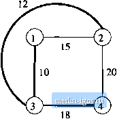

Figure 10.1: A graph; its minimum-weight spanning tree is indicated by heavy lines

J, B. Kruskal Jr., On the shortest spanning subtree of a graph and tho traveling salesman problem, Proc. A MS 7:1 (1956), pp. 48-50.

There is a well-known greedy algorithm, called Kruskals Algorithm, for finding a MWST. Here is an informal outline of the key ideas:

1. Maintain for each node the connected component in which the node appears, using whatever edges of the tree have been selected so far. Initially, no edges are selected, so every node is then in a connected component by itself.

2. Consider the lowest-weight edge that has not yet been considered; break ties any way you like. If this edge connects two nodes that are currently in different connected components then:

(a) Select that edge for the spanning tree, and

(b) Merge the two connected components involved, by changing the component number of all nodes in one of the two components to be the same as the component number of the other.

If, on the other hand, the selected edge connects two nodes of the same component, then this edge does not belong in the spanning tree; it would create a cycle.

3. Continue considering edges until either all edges have been considered, or the number of edges selected for the spanning tree is one less than the number of nodes. Note that in the latter case, all nodes must be in one connected component, and we can stop considering edges.

Example 10.1: In the graph of Fig. 10.1, we first consider the edge (1,3), because it has the lowest weight, 10. Since 1 Md 3 are initially in different components, we accept this edge, and make 1 and 3 have the same component number, say component 1. The next edge in order of weights is (2,3), with weight 12. Since 2 and 3 are in different components, we accept this edge and merge node 2 into component 1. The third edge is (1,2), with weight 15. However, 1 and 2 are now in the same component, so we reject this edge and proceed to the fourth edge, (3,4), Since 4 is not in component 1, we accept this edge. Now, we have three edges for the spanning tree of a 4-node graph, and so may stop. □

It is possible to implement this algorithm (using a computer, not a Turing machine) on a graph with m nodes and e edges in time 0{m + e\oge). A simpler, easier-to-follow implementation proceeds in e rounds, A table gives the current component of each node. We pick the lowest-weight remaining edge in 0(e) time, and find the components of the two nodes connected by the edge in 0{m) time. If they are in different components, merge all nodes with those numbers in 0{m) time, by scanning the table of nodes. The total time taken