1 Л

2 -2

I. J

4 /S

Figure 11.4: Tape of a DTM simulating a NTM by recursive calls to reach

While it may appear that many calls to reach are possible, and the tape of Fig. 11.4 can become very long, we shall show that it cannot become too long. That is, if started with a move count of m, there can only be loga m stack frames on the tape at any one time. Since Theorem 11.4 assures us that the NTM N cannot make more than c moves, m does not have to start with a number greater than that. Thus, the number of stack frames is at most loggc , which is 0[p{n)). We now have the essentials behind the proof of the following theorem.

Theorem 11.5: (Savitchs Theorem] PS = AfPS.

PROOF: It is obvious that VS С AfVS., since every DTM is technically a NTM as well. Thus, we need only to show that J\/VS Q VS; that is, if L is accepted by some NTM Л with space bound p{ri), for some polynomial p{n], then L is also accepted by some DTM D with polynomial space bound q{n), for some other polynomial q{n). In fact, we shall show that q{n) can be chosen to be on the order of the square of p{n).

First, we may assume by Theorem 11.3 that if N accepts, it does so within i+p[n) gj;gpg foj- gomc constant c. Given input w of length n, D discovers what N does with input w by repeatedly placing the triple [lo, J,m] on its tape and calUng reach with these arguments, where:

1. 7o is the initial ID of N with input w.

2. J is any accepting ID that uses at most p{n) tape cells; the different Js are enumerated systematically by using a scratch tape.

3. m - f:i+P( ).

We argued above that there will never be more than logg m recursive calls that are active at the same time, i.e., one with third argument m, one with m/2, one with m/4, and so on, down to 1. Thus, there are no more than log m stack frames on the stack, and loggm is 0{p{n)).

Further, the stack frames themselves take 0{p(n)) space. The reason is that the two IDS each require only 1 + p{n) cells to write down, and if we write m

on, until at some point the third argument becomes 1. At that point, reach can apply the basis step, and needs no more recursive calls. It tests if / = J or /1- ,/, returning TRUE if either holds and FALSE if neither does. Figure 11.4 suggests what the stack of the DTM D looks like when there are as many active calls to reach as possible, given an initial move count of m.

in binary, it requires = log2 0 * cells, which is 0[p{n]). Thus, the entire stack frame, consisting of two IDs and an integer, takes 0{p{n)) space.

Since D can have 0{p{n)) stack frames at most, the total amount of space used is 0(p{n)). This amount of space is a polynomial if p{n) is polynomial, so we conclude that L has a DTM that is polynomial-space bounded. □

In summary, we can extend what we know about complexity classes to include the polynomial-space classes. The complete diagram is shown in Fig. 11.5.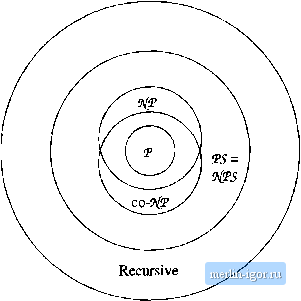

Figure 11.5: Known relationships among classes of languages

11.3 A Problem That Is Complete for VS

In this section, we shall introduce a problem called quantified boolean formulas and show that it is complete for PS.

11.3.1 PS-Completeness

We define a problem P to be complete for PS (PS-complete) if:

1. P is in PS.

2. All languages L in PS are polynomial-time reducible to P.

Notice that, although we are thinking about polynomial space, not time, the requirement for PS-completeness is similar to the requirement for NP-completeness: the reduction must be performed in polynomial time. The reason is that we want to know that, should some PS-complete problem turn out to be in V, then V = VS, and also if some PS-complete problem is in AfP, then AfV = VS. If the reduction were only in polynomial space, then the size of the output might be exponential in the size of the input, and therefore we could not draw the conclusions of the following theorem. However, since we focus on polynomial-time reductions, we get the desired relationships.

Theorem 11,6: Suppose P is a PS-complete problem. Then:

a) If P is in V, then V = VS.

b) If P is in AfV, then AfV = VS.

PROOF: Let us prove (a). For any L in VS, we know there is a polynomial-time reduction of L to P. Let this reduction take time q{n). Also, suppose P is in P, and therefore has a polynomial-time algorithm; say this algorithm runs in time pin).

Given a string w, whose membership in L we wish to test, we can use the reduction to convert it to a string x that is in P if and only if w is in L. Since the reduction takes time qiduil), the string x cannot be longer than We

may test membership of a: in P in time p(a;), which is p{qi\w\)), a polynomial in We conclude that there is a polynomial-time algorithm for L.

Therefore, every language L in VS is in P. Since containment of V in VS is obvious, we conclude that if P is in V, then V = VS. The proof for (b), where P is in AfV, is quite similar, and we shall leave it to the reader. □

11.3.2 Quantified Boolean Formulas

We are going to exhibit a problem P that is complete for VS. But first, we need to learn the terms in which this problem, called quantified boolean formulas or QBF, is defined.

Roughly, a quantified boolean formula is a boolean expression with the addition of the operators V ( for all ) and 3 ( there exists ). The expression iVx)iE) means that E is true when all occurrences of a: in S are replaced by 1 (true), and also true when all occurrences of x are replaced by 0 (false). The expression (Эж) (£) means that E is true either when all occurrences of x are replaced by 1 or when all occurrences of x are replaced by 0, or both.

To simplify our description, we shall assume that no QBF contains two or more quantifications (V or 3) of the same variable x. This restriction is not essential, and corresponds roughly to disallowing two different functions in a program firom using the same local variable. Formally, the quantified boolean

We can always rename one of two distinct uses of the same variable name, either in programs or in quantified boolean formulas. For programs, there is no reason to avoid reuse of the same local name, but in QBFs we find it convenient to assume there is no reuse.